API Reference
Everything documented here is part of the API, (except for things that are explicitly declared experimental), including the names that are not exported but do have docstrings. In Julia versions that support the public keyword, those unexported but public names are marked explicitly.
Design Problems
Specifying and Composing Design Problems
Kirstine.AbstractDesignProblem — Type
Kirstine.AbstractDesignProblemSupertype for all kinds of design problems.
See also DesignProblem, CompositeDesignProblem.
Kirstine.DesignProblem — Type
DesignProblem <: Kirstine.AbstractDesignProblemA DesignProblem has 7 components:
- a
DesignCriterion, - a
DesignRegion, - a
Model, - a
CovariateParameterization, - some
PriorKnowledge, - a
Transformation, - and a
NormalApproximation.
See also solve, and the mathematical background.
Kirstine.DesignProblem — Method
DesignProblem(<keyword arguments>)Construct a design problem with some sensible defaults.
Arguments
criterion::Kirstine.DesignCriterionregion::Kirstine.DesignRegionmodel::Kirstine.Modelcovariate_parameterization::Kirstine.CovariateParameterizationprior_knowledge::Kirstine.PriorKnowledgetransformation::Kirstine.Transformation = Identity()normal_approximation::Kirstine.NormalApproximation = FisherMatrix()
Kirstine.DesignProblem — Method
DesignProblem(prototype::DesignProblem; <keyword arguments>)Construct a design problem with defaults from prototype.
All explicitly given keyword arguments will be part of the new design problem. For every missing keyword argument, the corresponding field from prototype is copied instead. Note that the result does not share memory with prototype.
This function is useful for constructing variations of a given problem without having to retype a lot of code or having to write helper functions.
Examples
Consider some design problem
dp = DesignProblem(; criterion = DCriterion(), other_keyword_arguments...)This constructs a similar problem where only the criterion differs:
DesignProblem(dp; criterion = ACriterion())Kirstine.criterion — Function
Kirstine.region — Method
Kirstine.model — Function
Kirstine.covariate_parameterization — Function
Kirstine.prior_knowledge — Function
Kirstine.transformation — Function
Kirstine.normal_approximation — Function
Several AbstractDesignProblems can be combined to form a composite design problem, where a weighted sum of the component objectives is maximized. Composite design problems can be nested within each other.
Kirstine.CompositeDesignProblem — Type
CompositeDesignProblem <: Kirstine.AbstractDesignProblemA weighted construct of other abstract design problems.
See the mathematical background.
sourceKirstine.CompositeDesignProblem — Method
CompositeDesignProblem(problems, weights)Construct a composite design problem from a vector of AbstractDesignProblems and corresponding nonnegative weights.
All problems must have the same DesignRegion.
CompositeDesignProblems can be nested.
See also problems, weights(::CompositeDesignProblem), region(::CompositeDesignProblem).
Kirstine.problems — Method
Kirstine.weights — Method
weights(cdp::CompositeDesignProblem)Get the weights associated with the component design problems.
sourceKirstine.region — Method
region(cdp::CompositeDesignProblems)Get the common DesignRegion of the component design problems.
Solving Design Problems
Different high-level strategies are available for trying to solve any AbstractDesignProblem.
Kirstine.solve — Function
solve(
    adp::Kirstine.AbstractDesignProblem,
    strategy::Kirstine.ProblemSolvingStrategy;
    trace_state = false,
    sargs...,
)
Return a tuple (d, r).
d: The bestDesignMeasurefound. As postprocessing,simplifyandsort_pointsare called. Their respective keyword arguments can be mixed insargs, sincesolvewill take care to pass them along correctly.r: A subtype ofProblemSolvingResultthat is specific to the strategy used. Iftrace_state=true, this object contains additional debugging information. The unsimplified version ofdcan be accessed assolution(r).
See also DirectMaximization, Exchange.
Kirstine.DirectMaximization — Type
DirectMaximization <: Kirstine.ProblemSolvingStrategyFind an optimal design by directly maximizing a criterion's objective function.
sourceKirstine.DirectMaximization — Method
DirectMaximization(;
    optimizer::Kirstine.Optimizer,
    prototype::DesignMeasure,
    fixedweights = [],
    fixedpoints = [],
)
Initialize the optimizer with a single prototype and attempt to directly maximize the objective function.
For every index in fixedweights, the corresponding weight of prototype is held constant during optimization. The indices in fixedpoints do the same for the design points of the prototype. These additional constraints can be used to speed up computation in cases where some weights or design points are know analytically.
For more details on how the prototype is used, see the specific Optimizers.
The return value of solve for this strategy is a DirectMaximizationResult.
Kirstine.DirectMaximizationResult — Type
Kirstine.DirectMaximizationResult <: Kirstine.ProblemSolvingResultWraps the OptimizationResult from direct maximization.
See also solution(::DirectMaximizationResult), optimization_result.
Kirstine.solution — Method
Kirstine.total_runtime — Method
total_runtime(dmr::Kirstine.DirectMaximizationResult)Get the total time spent during optimization.
sourceKirstine.optimization_result — Function
Kirstine.Exchange — Type
Kirstine.Exchange — Method
Exchange(;
    optimizer_direction::Kirstine.ZerothOrderOptimizer,
    optimizer_weight::Kirstine.Optimizer,
    steps::Integer,
    gateaux_tolerance::Real,
    initial_weight::Real,
    candidate::DesignMeasure,
    simplify_args = Dict{Symbol,Any}(),
)
Improve the initial candidate design by repeating the following in a loop at most steps times:
- Recompute optimal weights for the current
candidatewhile keeping all points fixed. simplifythe currentcandidate, passing alongsimplify_args.- Find the one-point design
dtowards which thegateauxderivativeat the currentcandidateis largest. This usesoptimizer_direction, initialized with one-point prototypes at thepointsof the currentcandidate. See the low-levelOptimizers for algorithm-specific details. - If the maximum Gateaux derivative is smaller than or equal to
gateaux_tolerance, stop early. - Append the single point of
dto the support of the currentcandidateand give itinitial_weight, scaling down the already existing by1-initial_weight. In the special caseinitial_weight=NaN, the weight of the new point is set to1/(1 + points(candidate)).
Note that depending on the chosen optimizers, this strategy can produce intermediate designs with a lower value of the objective function than the candidate you started with.
The return value of solve for this strategy is an ExchangeResult.
Before version 0.8.0 of Kirstine.jl, the order of the reweighting step and the derivative-maximizing step were swapped and initial_weight = NaN had been hard-coded
Kirstine.ExchangeResult — Type
Kirstine.ExchangeResult <: Kirstine.ProblemSolvingResultWraps the OptimizationResults from the individual steps.
See also solution(::ExchangeResult), optimization_results_direction, optimization_results_weight.
Kirstine.solution — Method
Kirstine.total_runtime — Method
Kirstine.total_runtime_direction — Method
total_runtime_direction(er::Kirstine.ExchangeResult)Get the total time spent during the direction steps.
sourceKirstine.total_runtime_weight — Method
total_runtime_weight(er::Kirstine.ExchangeResult)Get the total time spent during the reweighting steps.
sourceKirstine.optimization_results_direction — Function
optimization_results_direction(er::Kirstine.ExchangeResult)Get the vector of OptimizationResults from the direction steps.
Kirstine.optimization_results_weight — Function
optimization_results_weight(er::Kirstine.ExchangeResult)Get the full OptimizationResults from the reweighting steps.
Particle-based optimizers are operating on a lower level, and are used as part of a Kirstine.ProblemSolvingStrategy.
Kirstine.Optimizer — Type
Kirstine.OptimizerSupertype for particle-based optimization algorithms.
See also Pso, GridSearch, FrankWolfe.
Kirstine.ZerothOrderOptimizer — Type
Kirstine.ZerothOrderOptimizer <: Kirstine.OptimizerSupertype for optimization algorithms that only use the objective function.
sourceKirstine.FirstOrderOptimizer — Type
Kirstine.FirstOrderOptimizer <: Kirstine.OptimizerSupertype for optimization algorithms that use the objective function and its gradient.
sourceKirstine.OptimizationResult — Type
Kirstine.OptimizationResultWrapper for results of particle-based optimization.
Kirstine.OptimizationResult fields
| Field | Description |
|---|---|
| maximizer | final maximizer |
| maximum | final objective value |
| trace_x | vector of current maximizer in each iteration |
| trace_fx | vector of current objective value in each iteration |
| trace_gx | vector of current gradient in each iteration |
| trace_state | vector of internal optimizer state in each iteration |
| has_converged | true if the algorithm has converged |
| n_eval_f | total number of objective evaluations |
| n_eval_g | total number of gradient evaluations |
| seconds_elapsed | total runtime |
Note that for a ZerothOrderOptimizer trace_gx will be empty and n_eval_g == 0.
See also solve.
Kirstine.Pso — Type
Pso <: Kirstine.ZerothOrderOptimizerA constricted particle swarm optimizer.
There is a large number of published PSO variants, this one was taken from two [CK02] publications [ES00].
Note that particle swarm optimization has no convergence guarantees, hence the has_converged field of the OptimizationResult returned by a PSO run is always false by definition.
Initialization
The swarm is initialized from a vector of prototypical AbstractPoints, which are supplied by the caller via a nonexported interface. Construction from the vector of prototypes proceeds as follows:
The first
length(prototypes)particles are a deep copy of theprototypesvector.Each of the remaining particles is a deep copy of
prototypes[1]which is subsequently randomized. Randomization is subject to constraints, if any are given.
Kirstine.Pso — Method
Pso(; iterations, swarmsize, c1 = 2.05, c2 = 2.05)Set up parameters for a particle swarm optimizer.
c1 controls movement towards a particle's personal best, while c2 controls movement towards the global best. In this implementation, a particle's neighborhood is the whole swarm.
Kirstine.GridSearch — Type
GridSearch <: Kirstine.ZerothOrderOptimizerA grid search optimizer.
This optimizer is particularly useful for the direction-finding step in Exchange, but can also be used for DirectMaximization as long as all weights of the candidate are fixed, and there are only few nonfixed design points. Note that for DirectMaximization, the total number of grid points is exponential both in the dimension of the design region and in the number of nonfixed design points.
(Strictly speaking this optimizer is not particle-based, but it uses the same internal infrastructure.)
Since grid search finds the maximum over a finite set of points, the has_converged flag of a corresponding OptimizationResult is always true by definition.
Initialization
Similar to optimization with Pso, the optimizer state is initialized internally with a vector of prototype points. The first prototype determines the structure of each grid point that is constructed from the Kirstine.GridSpec. This set of points is then merged with the vector of prototypes and used for maximization.
Kirstine.GridSearch — Method
GridSearch(; gridspec::Kirstine.GridSpec)Set up parameters for a grid search.
The GridSpec is used to construct a grid over the problem's DesignRegion, so the dimensions of both must be equal.
Examples
julia> GridSearch(; gridspec = ProductGrid(11, 11))
GridSearch{ProductGrid{2}}(ProductGrid{2}((11, 11)))Kirstine.GridSpec — Type
Kirstine.ProductGrid — Type
ProductGrid <: Kirstine.GridSpecA Cartesian product with the given number of grid points in each dimension.
Examples
A 2-dimensional grid with 5×11 points:
julia> ProductGrid(5, 11)
ProductGrid{2}((5, 11))Kirstine.FrankWolfe — Type
FrankWolfe <: Kirstine.FirstOrderOptimizerA Frank-Wolfe optimizer.
Two variants are implemented: a basic one that always moves towards the best vertex for the linearized problem (see Algorithm 4 in [P23]), and a version with pairwise steps (see Algorithm 2 in [LJ15]) that is better at finding an optimum on the boundary.
It is currently intended to be used for the reweighting step of Exchange. For DirectMaximization it can currently only be used when all design points are fixed.
Initialization
Frank-Wolfe can only be initialized with a single prototype. This prototype will be used as the starting value.
sourceKirstine.FrankWolfe — Method
FrankWolfe(; iterations::Integer, fw_gap_tolerance::Real, stepsize::StepSizeStrategy, pairwise::Bool)Set up parameters for the Frank-Wolfe algorithm. The argument iterations sets the maximum number of iterations to run. The algorithm terminates early if the Frank-Wolfe gap of the current iteration is smaller than or equal to the given tolerance.
Kirstine.StepSizeStrategy — Type
Kirstine.OpenLoop — Type
OpenLoop <: Kirstine.StepSizeStrategy
OpenLoop(; shift = 2)
Frank-Wolfe step-size strategy $γ(t) = l / (t + l)$ for $t=0,1,2,…$ with shift $l∈ℕ, l≥1$.
With OpenLoop, the algorithm will always land on a vertex of the feasible set at $t=1$. For a probability simplex, these vertices are the one-point designs. As a consequence, OpenLoop is not suitable for the reweighting step of Exchange for design problems where one-point designs are singular.
Kirstine.ConstNumIter — Type
ConstNumIter <: Kirstine.StepSizeStrategyFrank-Wolfe step-size strategy $γ(t) = 1 / \sqrt{T}$ for a run with $T$ iterations $t=0,…,T-1$.
sourceKirstine.Adaptive — Type
Adaptive <: Kirstine.StepSizeStrategy
Adaptive(; eta = 0.9, tau = 2.0, initial_smoothness_estimate = Inf, smoothness_threshold = 1e10)
Adaptive Frank-Wolfe step-size strategy that uses a smoothness property of the objective function.
Since we typically do not know the smoothness constant of the objective function $f$, i.e. a real number $L$ such that $⟨∇f(y) - ∇f(x), y - x⟩ ≤ L\lVert y-x\rVert^2$ for all $x$ and $y$ in the convex domain of $f$, the constant is dynamically approximated via multiplicative search with parameters eta ≤ 1 and tau > 1. When initial_smoothness_estimate = Inf, the initial estimate is computed from a local approximation at the starting value.
If at any point during the search the smoothness estimate exceeds smoothness_threshold, this is interpreted as the divergence of the multiplicative search, and the current (nonoptimal) step size is returned.
This strategy is an implementation of Algorithm 5 from [P23], and the defaults of the parameters are taken from the adaptive line search in FrankWolfe.jl.
sourceDesign Criteria
Kirstine.DesignCriterion — Type
Kirstine.DesignCriterionSupertype for optimal experimental design criteria.
See also DCriterion, ACriterion.
Kirstine.DCriterion — Type
DCriterion <: Kirstine.DesignCriterionCriterion for D-optimal experimental design.
Log-determinant of the normalized information matrix.
See also the mathematical background.
sourceKirstine.ACriterion — Type
ACriterion <: Kirstine.DesignCriterionCriterion for A-optimal experimental design.
Trace of the inverted normalized information matrix.
See also the mathematical background.
sourceKirstine.objective — Function
objective(d::DesignMeasure, adp::Kirstine.AbstractDesignProblem)Evaluate the objective function.
See also the mathematical background.
sourceKirstine.gateauxderivative — Function
gateauxderivative(
    at::DesignMeasure,
    towards::AbstractArray{DesignMeasure},
    dp::DesignProblem,
)
The designs towards which we compute the derivative are allowed to have different numbers of points.
See also the mathematical background.
sourceKirstine.max_argmax_gateauxderivative — Function
Kirstine.max_argmax_gateauxderivative(
    at::DesignMeasure,
    adp::AbstractDesignProblem;
    n_grid::Union{Integer,NTuple{N,Integer}}
)
Compute the maximal Gateaux derivative towards one-point designs from a grid over the design region.
The dimension of the DesignRegion of adp must equal N. The number of points in each dimension of the grid is given by the elements of n_grid. For convenience in case N==1, a single Integer can be given instead of a 1-tuple. If the design region is not an interval, the grid is constructed on the region's bounding box and grid points outside the region will be ignored.
Returns the maximum of the Gateaux derivative and the one-point design towards which the maximum is attained.
sourceKirstine.efficiency — Function
efficiency(d1::DesignMeasure, d2::DesignMeasure, dp::DesignProblem)
efficiency(d1::DesignMeasure, d2::DesignMeasure, dp1::DesignProblem, dp2::DesignProblem)
Relative efficiency of d1 to d2 under the corresponding problems.
The function with two design problems is only defined if there is a sensible notion of efficiency for the combination of the two DesignCriterion fields. For the DCriterion, the dimensions of the transformed parameters must be identical. Apart from that, the two design problems are allowed to be completely different. The function with three arguments is a shorthand for when dp1 and dp2 are identical.
See also the mathematical background.
Before version 0.8.0 of Kirstine.jl, the criteria of the design problems were ignored and D-efficiency was computed unconditionally. The old behavior can be mimicked by explicitly calling
efficiency(d1, d2, DesignProblem(dp1; criterion = DCriterion()), DesignProblem(dp2; criterion = DCriterion()))Kirstine.shannon_information — Function
shannon_information(d::DesignMeasure, dp::DesignProblem, n::Integer)Compute the approximate expected posterior Shannon information for an experiment with n units of observation under design d and design problem dp.
See also the mathematical background.
dis notapportioned.- Shannon information is motivated by D-optimal design, so this function ignores the type of
criterion(dp).
Design Regions
Kirstine.DesignRegion — Type
Kirstine.DesignRegion{N}Supertype for design regions. A design region is a compact subset of $\Reals^N$.
The design points of a DesignMeasure are taken from this set.
See also DesignInterval, dimnames.
Kirstine.DesignInterval — Type
DesignInterval{N} <: Kirstine.DesignRegion{N}A (hyper)rectangular subset of $\Reals^N$.
See also lowerbound, upperbound, dimnames.
Kirstine.DesignInterval — Method
DesignInterval(names, lowerbounds, upperbounds)Construct a design interval.
Examples
julia> DesignInterval([:dose, :time], [0, 0], [300, 20])
DesignInterval(:dose => (0.0, 300.0), :time => (0.0, 20.0))Kirstine.DesignInterval — Method
DesignInterval(name_bounds::Pair...)Construct a design interval from name => (lb, ub) pairs for individual dimensions.
Note that the order of the arguments matters and that it should match the implementation of map_to_covariate! for your Model and Covariate subtypes.
Examples
julia> DesignInterval(:dose => (0, 300), :time => (0, 20))
DesignInterval(:dose => (0.0, 300.0), :time => (0.0, 20.0))Kirstine.dimension — Method
Kirstine.dimnames — Function
Kirstine.upperbound — Function
Kirstine.lowerbound — Function
Nonlinear Regression Models
Regression models are implemented by first subtyping Kirstine.Model, Kirstine.Covariate, Kirstine.CovariateParameterization, and Kirstine.Parameter, and then defining several helper methods on them.
For models with a scalar-valued unit of observation and for parameters that are a collection of scalar values, this can easily be achieved with the @simple_model and @simple_parameter macros. See the tutorial for a hands-on example and the section on helpers below. For an example of a manually implemented model see the dose-time-response vignette, and for both a manual model and a manual parameter the vignette on automatic differentiation.
Supertypes
Kirstine.Model — Type
Kirstine.NonlinearRegression — Type
Kirstine.Covariate — Type
Kirstine.CovariateSupertype for user-defined model covariates.
Implementation
Subtypes of Kirstine.Covariate should be mutable, or have at least a mutable field. This is necessary for being able to modify them in map_to_covariate!.
Kirstine.CovariateParameterization — Type
Kirstine.CovariateParameterizationSupertype for user-defined mappings from design points to model covariates.
See also implied_covariates.
Kirstine.Parameter — Type
Implementing a Nonlinear Regression Model
Suppose the following subtypes have been defined:
M <: Kirstine.NonlinearRegressionC <: Kirstine.CovariateCp <: Kirstine.CovariateParameterizationP <: Kirstine.Parameter
Then methods need to be added for the following package-internal functions:
Kirstine.allocate_covariate — Function
Kirstine.allocate_covariate(m::M) -> c::CConstruct a single covariate for the model.
Implementation
For user types M <: Kirstine.Model and a corresponding C <: Kirstine.Covariate, this should construct a single instance c of C with some (model-specific) sensible initial value.
See also the mathematical background.
sourceKirstine.jacobianmatrix! — Function
Kirstine.jacobianmatrix!(jm::AbstractMatrix{<:Real}, m::M, c::C, p::P) -> jmCompute Jacobian matrix of the mean function at p.
Implementation
For user types M <: Kirstine.NonlinearRegression, C <: Kirstine.Covariate, and P <: Kirstine.Parameter, this should fill in the elements of the preallocated Jacobian matrix jm, and finally return jm.
Note that you are free how you map the partial derivatives to the columns of jm. The only thing that is required is to use the same order in any DeltaMethod that you want to implement.
See also the mathematical background.
sourceKirstine.map_to_covariate! — Function
Kirstine.map_to_covariate!(c::C, dp::AbstractVector{<:Real}, m::M, cp::Cp) -> cMap a design point to a model covariate.
Implementation
For user types C <: Kirstine.Covariate, M <: Kirstine.Model, and Cp <: Kirstine.CovariateParameterization this should set the fields of the single covariate c according to the single design point dp. Finally, this method should return c.
See also implied_covariates and the mathematical background.
Kirstine.update_model_vcov! — Function
Kirstine.update_model_vcov!(Sigma::Matrix, m::M, c::C)Compute variance-covariance matrix of the nonlinear regression model for one unit of observation.
Implementation
For user types C <: Kirstine.Covariate and M <: Kirstine.NonlinearRegression, this should fill in the elements of Sigma for a unit of observation with covariate c. The size of the matrix is (unit_length(m), unit_length(m)).
See also the mathematical background.
sourceKirstine.unit_length — Function
Kirstine.unit_length(m::M) -> IntegerReturn the length of one unit of observation.
Implementation
For a user type M <: Kirstine.Model this should return the length $\DimUnit$ of one unit of observation $\Unit$.
See also the mathematical background.
sourceKirstine.dimension — Function
Kirstine.dimension(p::P) -> IntegerReturn dimension of the parameter space.
Implementation
For a user type P <: Kirstine.Parameter, this should return the dimension of the parameter space.
See also the mathematical background.
sourceSome of these methods only require M <: Kirstine.Model and not M <: Kirstine.NonlinearRegression. This is intentional. These methods can in principle also be implemented for M <: Ma where abstract type Ma <: Kirstine.Model end is also user-defined.
Helpers
To reduce boilerplate code in the common cases of a one-dimensional unit of observation, and for a vector parameter without any additional structure, the following helper macros can be used:
Kirstine.@simple_model — Macro
@simple_model name covariate_field_names...Generate code for defining a NonlinearRegression model, a corresponding Covariate, and helper functions for a 1-dimensional unit of observation with constant measurement variance.
This macro will define the two types $(name)Model and $(name)Covariate, hence name should start with a capital letter. The model constructor will have the measurement standard deviation sigma as a mandatory argument.
Examples
The call
@simple_model Emax doseis equivalent to manually spelling out
@kwdef struct EmaxModel <: Kirstine.NonlinearRegression
    sigma::Float64
    function EmaxModel(sigma::Real)
        if sigma <= 0
            throw(ArgumentError("sigma must be positive"))
        end
        return new(sigma)
    end
end
mutable struct EmaxCovariate <: Kirstine.Covariate
    dose::Float64
end
Kirstine.unit_length(m::EmaxModel) = 1
function Kirstine.update_model_vcov!(Sigma::Matrix{Float64}, m::EmaxModel, c::EmaxCovariate)
    Sigma[1, 1] = m.sigma^2
    return Sigma
end
Kirstine.allocate_covariate(m::EmaxModel) = EmaxCovariate(0)
Note that this works both when you are using Kirstine and when you are importing it, even if you do something like
import Kirstine as SmithFurther note that the @simple_model macro can be used together with, or independently of @simple_parameter.
Kirstine.@simple_parameter — Macro
@simple_parameter name field_names...Generate code for defining a subtype of Parameter with the given name and fields, and define its dimension as length(field_names).
This macro will define the type $(name)Parameter, hence name should start with a capital letter. The type will have a keyword constructor. All fields will have the type Float64.
Examples
The call
@simple_parameter Emax e0 emax ec50is equivalent to
@kwdef struct EmaxParameter <: Kirstine.Parameter
    e0::Float64
    emax::Float64
    ec50::Float64
end

Kirstine.dimension(p::EmaxParameter) = 2
An EmaxParameter object with e0=1, emax=2, and ec50=4 can then be constructed by
EmaxParameter(; e0 = 1, emax = 2, ec50 = 4)Note that this works both when you are using Kirstine and when you are importing it, even if you do something like
import Kirstine as SmithFurther note that the @simple_parameter macro can be used together with, or independently of @simple_model.
In problems where the design variables coincide with the model covariates, the following Kirstine.CovariateParameterization can be used:
Kirstine.CopyTo — Type
CopyTo <: Kirstine.CovariateParameterizationA convenience type to use when design variables and model covariates are identical.
sourceKirstine.CopyTo — Method
CopyTo(names::Symbol...)Construct a CovariateParameterization that copies the elements of a design point to the fields of a Covariate with the given names.
This parameterization can be used with any Covariate that has only Float64 fields. Note that the order of the names should match the order of dimnames(region(prob)) for the DesignProblem in which CopyTo is used. No new method for map_to_covariate! needs to be implemented for user types since the package supplies a generic one that works with any Model and any Covariate.
See also the tutorial for another usage example.
Examples
When we have
julia> @simple_model Foo a b

julia> @simple_parameter Foo θ
we can define
julia> cp = CopyTo(:a, :b)
CopyTo(:a, :b)
and then solve
julia> dp = DesignProblem(;
           region = DesignInterval(:a => (0, 1), :b => (-2, 5)),
           covariate_parameterization = cp,
           criterion = DCriterion(),
           model = FooModel(; sigma = 1),
           prior_knowledge = PriorSample([FooParameter(; θ = 42)]),
       );
whithout first having to add a method to map_to_covariate! for the FooModel and FooCovariate types.
Note however that the equivalent manual version
julia> struct CopyBoth <: Kirstine.CovariateParameterization end

julia> function Kirstine.map_to_covariate!(c::FooCovariate, dp, m::FooModel, cp::CopyBoth)
           c.a = dp[1]
           c.b = dp[2]
           return c
       end
would be slightly more efficient since it knows the types and field names at compile time.
Also note that since the design points are assigned in the order of the names given, cp = CopyTo(:b, :a) would be equivalent to setting c.b = dp[1] and c.a = dp[2].
Prior Knowledge
Kirstine.PriorKnowledge — Type
Kirstine.PriorKnowledge{T<:Kirstine.Parameter}Supertype for representing prior knowledge of the model Parameter.
See also PriorSample.
Kirstine.PriorSample — Type
PriorSample{T} <: Kirstine.PriorKnowledge{T}A sample from a prior distribution, or a discrete prior distribution with finite support.
sourceKirstine.PriorSample — Method
PriorSample(p::AbstractVector{<:Kirstine.Parameter} [, weights::AbstractVector{<:Real}])Construct a weighted prior sample on the given parameter draws.
If no weights are given, a uniform distribution on the elements of p is assumed.
See also parameters, weights(::PriorSample).
Base.:== — Method
==(pk1::PriorSample, pk2::PriorSample)Test prior samples for equality.
Two prior samples are considered equal iff
- they have the same subtype of
Parameter, - and their parameter draws are equal,
- and their weights are equal,
- and the order of the draws is equal.
Note that this is stricter than when comparing prior samples as mathematical sets, where the order of the draws does not matter.
sourceKirstine.parameters — Method
parameters(pk::PriorSample)Return a reference to the parameters of the PriorSample.
See also weights(::DesignMeasure).
Kirstine.weights — Method
weights(pk::PriorSample)Return a reference to the weights of the PriorSample.
See also parameters.
Transformations
Kirstine.Transformation — Type
Kirstine.TransformationSupertype of posterior transformations.
See also Identity, DeltaMethod, and the mathematical background.
Kirstine.Identity — Type
Kirstine.DeltaMethod — Type
DeltaMethod <: Kirstine.Transformation
DeltaMethod(jacobian_matrix::Function)
A nonlinear Transformation of the model parameter.
The delta method uses the Jacobian matrix $\TotalDiff\Transformation$ to map the asymptotic multivariate normal distribution of $\Parameter$ to the asymptotic multivariate normal distribution of $\Transformation(\Parameter)$.
To construct a DeltaMethod object, jacobian_matrix must be a function that maps a Parameter p to the Jacobian matrix of $\Transformation$ evaluated at p.
Note that the order of the columns must match the order that you used when implementing the jacobianmatrix! for your model.
The Dimension of the Transformed Parameter
Several places in the package need to know the dimension of $\Transformation(\Parameter)$. By default, this will be computed by evaluating $\TotalDiff\Transformation(\Parameter)$ for one $\Parameter$ from the prior sample, and then counting the number of rows of this matrix. However, this may be undesirable when $\TotalDiff\Transformation$ is expensive to compute (e.g., when it requires numerical integration). To prevent this default behavior, you can implement a method for the internal function transformed_parameter_dimension that dispatches on the types of your jacobian_matrix function and your model parameter.
For example, suppose you have an 8-dimensional MyParameter <: Parameter and an expensive transformation to something 5-dimensional. Then you would write
function expensive_dt(p::MyParameter)
    # some expensive computations that return a matrix with size (5, 8)
end
function Kirstine.transformed_parameter_dimension(dt::typeof(expensive_dt), p::MyParameter)
    return 5
end
Examples
Suppose p has the fields a and b, and $\Transformation(\Parameter) = (ab, b/a)'$. Then the Jacobian matrix of $\Transformation$ is
\[\TotalDiff\Transformation(\Parameter) = \begin{bmatrix} b & a \\ -b/a^2 & 1/a \\ \end{bmatrix}.\]
In Julia this is equivalent to
jm1(p) = [p.b p.a; -p.b/p.a^2 1/p.a]
DeltaMethod(jm1)
Note that for a scalar quantity, e.g. $\Transformation(\Parameter) = \sqrt{ab}$, the Jacobian matrix is a row vector.
jm2(p) = [b a] ./ (2 * sqrt(p.a * p.b))
DeltaMethod(jm2)Normal Approximations
Kirstine.NormalApproximation — Type
Kirstine.NormalApproximationSupertype for different possible normal approximations to the posterior distribution.
sourceKirstine.FisherMatrix — Type
FisherMatrixNormal approximation based on the maximum-likelihood approach.
The information matrix is obtained as the average of the Fisher information matrix with respect to the design measure. Singular information matrices can occur.
See also the mathematical background.
sourceDesign Measures
Kirstine.DesignMeasure — Type
DesignMeasureA probability measure with finite support representing a continuous experimental design.
The support points of a design measure are called design points. In Julia, a design point is simply a Vector{Float64}.
Special kinds of design measures can be constructed with one_point_design, uniform_design, equidistant_design, random_design.
See also weights(::DesignMeasure), points, apportion, plotting API.
Base.:== — Method
==(d1::DesignMeasure, d2::DesignMeasure)Test design measures for equality.
Two design measures are considered equal iff
- they have the same number of design points,
- and their design points and weights are equal,
- and their design points are in the same order.
Note that this is stricter than when comparing measures as mathematical functions, where the order of the design points in the representation does not matter.
sourceKirstine.DesignMeasure — Method
DesignMeasure(
    points::AbstractMatrix{<:Real},
    weights::AbstractVector{<:Real}
)
Construct a design measure with design points from the columns of points.
This is the only design measure constructor where the result does share memory with points and weights.
Kirstine.DesignMeasure — Method
DesignMeasure(
    points::AbstractVector{<:AbstractVector{<:Real}},
    weights::AbstractVector{<:Real},
)
Construct a design measure from a vector of design points.
The result does not share memory with points.
Examples
julia> DesignMeasure([[1, 2], [3, 4], [5, 6]], [0.5, 0.2, 0.3])
DesignMeasure(
 [1.0, 2.0] => 0.5,
 [3.0, 4.0] => 0.2,
 [5.0, 6.0] => 0.3,
)Kirstine.DesignMeasure — Method
DesignMeasure(dp_w::Pair...)Construct a design measure from designpoint => weight pairs.
Examples
julia> DesignMeasure([1] => 0.2, [42] => 0.3, [9] => 0.5)
DesignMeasure(
 [1.0] => 0.2,
 [42.0] => 0.3,
 [9.0] => 0.5,
)Kirstine.one_point_design — Function
one_point_design(designpoint::AbstractVector{<:Real})Construct a one-point DesignMeasure.
The result does not share memory with designpoint.
Examples
julia> one_point_design([42])
DesignMeasure(
 [42.0] => 1.0,
)Kirstine.uniform_design — Function
uniform_design(designpoints::AbstractVector{<:AbstractVector{<:Real}})Construct a DesignMeasure with equal weights on the given designpoints.
The result does not share memory with designpoints.
Examples
julia> uniform_design([[1], [2], [3], [4]])
DesignMeasure(
 [1.0] => 0.25,
 [2.0] => 0.25,
 [3.0] => 0.25,
 [4.0] => 0.25,
)Kirstine.equidistant_design — Function
equidistant_design(dr::DesignInterval{1}, K::Integer)Construct a DesignMeasure with an equally-spaced grid of K design points and uniform weights on the given 1-dimensional design interval.
Examples
julia> equidistant_design(DesignInterval(:z => (0, 1)), 5)
DesignMeasure(
 [0.0] => 0.2,
 [0.25] => 0.2,
 [0.5] => 0.2,
 [0.75] => 0.2,
 [1.0] => 0.2,
)Kirstine.random_design — Function
random_design(dr::Kirstine.DesignRegion, K::Integer)Construct a random DesignMeasure.
The design points are drawn independently from the uniform distribution on the design region, and the weights drawn from the uniform distribution on a simplex.
sourceKirstine.points — Function
points(d::DesignMeasure)Return an iterator over the design points of d.
See also weights(::DesignMeasure), numpoints.
Kirstine.weights — Method
Kirstine.numpoints — Function
numpoints(d::DesignMeasure)Return the number of design points of d.
See also points, weights(::DesignMeasure).
Kirstine.sort_points — Function
sort_points(d::DesignMeasure; rev = false, dimorder = 1:length(first(points(d))))Return a representation of d where the design points are sorted lexicographically.
By default, the result is sorted by the first dimension of the design points, and ties are resolved by the second, further ties by the third, and so on. This can be changed by setting dimorder to a different permutation.
See also sort_weights.
Examples
julia> sort_points(uniform_design([[3, 40], [2, 10], [1, 20], [2, 30]]))
DesignMeasure(
 [1.0, 20.0] => 0.25,
 [2.0, 10.0] => 0.25,
 [2.0, 30.0] => 0.25,
 [3.0, 40.0] => 0.25,
)

julia> sort_points(uniform_design([[3, 40], [2, 10], [1, 20], [2, 30]]); dimorder = [2, 1])
DesignMeasure(
 [2.0, 10.0] => 0.25,
 [1.0, 20.0] => 0.25,
 [2.0, 30.0] => 0.25,
 [3.0, 40.0] => 0.25,
)Kirstine.sort_weights — Function
sort_weights(d::DesignMeasure; rev::Bool = false)Return a representation of d where the design points are sorted by their corresponding weights.
See also sort_points.
Examples
julia> sort_weights(DesignMeasure([[1], [2], [3]], [0.5, 0.2, 0.3]))
DesignMeasure(
 [2.0] => 0.2,
 [3.0] => 0.3,
 [1.0] => 0.5,
)Kirstine.mixture — Function
mixture(alpha, d1::DesignMeasure, d2::DesignMeasure)Return the convex combination $α d_1 + (1-α) d_2$.
The result is not simplified, hence its design points might not be unique.
sourceKirstine.apportion — Function
Kirstine.simplify — Method
simplify(d::DesignMeasure, dp::DesignProblem; maxweight = 0, maxdist = 0, uargs...)A wrapper that calls simplify_unique, simplify_merge (with the design region of dp), and simplify_drop in that order.
Kirstine.simplify — Method
simplify(d::DesignMeasure, cdp::CompositeDesignProblem; maxweight = 0, maxdist = 0, uargs...)A wrapper that calls simplify_merge, and simplify_drop in that order.
Note that uargs are ignored since there is no obvious generalization of simplify_unique for general composite design problems. When uargs is not empty, a warning is printed.
Kirstine.simplify_drop — Function
simplify_drop(d::DesignMeasure, maxweight::Real)Construct a new DesignMeasure where all design points with weights smaller than or equal to maxweight are removed.
The vector of remaining weights is renormalized.
sourceKirstine.simplify_unique — Function
simplify_unique(d::DesignMeasure, dr::Kirstine.DesignRegion, m::M, cp::C; uargs...)Construct a new DesignMeasure that corresponds uniquely to its implied normalized information matrix.
The package default is a catch-all with the abstract types M = Model and C = CovariateParameterization, which simply returns a copy of d.
When called via simplify, user-model specific keyword arguments will be passed in uargs.
Implementation
Users can specialize this method for their concrete subtypes M <: Kirstine.Model and C <: Kirstine.CovariateParameterization. It is intended for cases where the mapping from design measure to normalized information matrix is not one-to-one. This depends on the model and covariate parameterization used. In such a case, simplify_unique should be implemented to select a canonical version of the design.
Examples
For several worked examples, see the dose-time-response vignette.
sourceKirstine.simplify_merge — Function
simplify_merge(d::DesignMeasure, dr::Kirstine.DesignRegion, maxdist::Real)Merge designpoints with a normalized distance smaller or equal to maxdist.
Special case of simplify_merge with f(z) = (z .- lb) ./ (ub .- lb), where ub and lb define the bounding box of dr, and distfun(x, y) = norm(x - y).
In other words, the design points of d are scaled into the N-dimensional unit cube before measuring their pairwise distances. Note that the largest possible distance between points is sqrt(N).
Examples
After scaling into the unit square, the distance between the first two points less than 0.3, hence they are merged.
julia> d = DesignMeasure([[2.25, 2], [3.5, 2.5], [10, 3]], [0.3, 0.1, 0.6]);

julia> simplify_merge(d, DesignInterval(:a => (1, 11), :b => (2, 4)), 0.3)
DesignMeasure(
 [2.5624999999999996, 2.125] => 0.4,
 [10.0, 3.0] => 0.6,
)simplify_merge(d::DesignMeasure, f::Function, distfun::Function, maxdist::Real)Merge design points with distfun(f(dp1), f(dp2)) smaller or equal to maxdist.
The following two steps are repeated until all points are more than maxdist apart:
- All pairwise distances are calculated.
- The two points closest to each other are averaged according to their relative weights.
Examples
The first example uses the 2-norm for measuring distances between the points directly, and merges the first two points since they are 1/sqrt(2) apart. The second example uses the 1-norm instead, where the first two points have distance 1, so nothing happens.
julia> d = DesignMeasure([[1, 2], [1.5, 2.5], [3, 3]], [0.1, 0.4, 0.5]);

julia> simplify_merge(d, identity, (x, y) -> sqrt(sum((x .- y) .^ 2)), 0.8)
DesignMeasure(
 [1.4000000000000001, 2.4] => 0.5,
 [3.0, 3.0] => 0.5,
)

julia> simplify_merge(d, identity, (x, y) -> sum(abs.(x - y)), 0.8)
DesignMeasure(
 [1.0, 2.0] => 0.1,
 [1.5, 2.5] => 0.4,
 [3.0, 3.0] => 0.5,
)
The third example has two pairs of points with the same distance to each other. When simplified with a design region, either none or both are merged. However, when mapped onto the graph of the exp() function, only the second pair will be merged since it is spread much wider than the first. Such a behavior might be desired with a more complicated expected response function in place of exp().
julia> d = uniform_design([[0.2], [0.3], [4.9], [5.0]]);

julia> simplify_merge(d, DesignInterval(:a => (0, 10)), 0.01)
DesignMeasure(
 [0.25] => 0.5,
 [4.95] => 0.5,
)

julia> simplify_merge(d, z -> [z[1], exp(z[1])], (x, y) -> sqrt(sum((x .- y) .^ 2)), 1)
DesignMeasure(
 [0.25] => 0.5,
 [4.9] => 0.25,
 [5.0] => 0.25,
)Kirstine.informationmatrix — Function
Kirstine.informationmatrix(
    d::DesignMeasure,
    m::Model,
    cp::Kirstine.CovariateParameterization,
    p::Kirstine.Parameter,
    na::Kirstine.NormalApproximation,
)
Compute the normalized information matrix for a single Parameter value p.
This function is useful for debugging.
See also apply_transformation and the mathematical background.
Kirstine.apply_transformation — Function
Kirstine.apply_transformation(nim::AbstractMatrix{<:Real}, p::Kirstine.Parameter, trafo::Kirstine.Transformation)Compute the information matrix for the transformed Parameter.
This function is useful for debugging.
See also informationmatrix and the mathematical background.
Kirstine.implied_covariates — Function
implied_covariates(d::DesignMeasure, m::M, cp::Cp)Return covariates that are implied by d for instances of user types M <: Kirstine.Model and Cp <: Kirstine.CovariateParameterization.
This function is useful for debugging.
See also map_to_covariate!.
Plotting
Kirstine.jl provides plot recipes for several (combinations of) types, instances of which can simply be plot()ted. For Gateaux derivatives and expected functions there are separate methods.
plot(d::DesignMeasure)
plot(d::DesignMeasure, dr::Kirstine.DesignRegion)
plot(r::Kirstine.OptimizationResult)
plot(rs::AbstractVector{<:OptimizationResult})
plot(r::Kirstine.DirectMaximizationResult)
plot(r::Kirstine.ExchangeResult)
The method for plotting DesignMeasures has several options.
- When a
DesignRegionis given,xlims(and for 2-dimensional design points alsoylims) is set to the boundaries of the region. - The
label_formatterkeyword argument accepts a function that maps a triple(k, pt, w)of an index, design point, and weight to a string. By default, the weight is indicated in percentage points rounded to 3 significant digits. Note that due to rounding the weights do not necessarily add up to 100%. To achieve this, consider plotting anapportioned version of your design measure like this:DesignMeasure(points(d), apportion(weights(d), 1000) ./ 1000) - The
maxmarkersizekeyword argument indicates themarkersize(radius in pixels) of a design point with weight 1. Other points are scaled down according to thesqrtof their weight. It will be overridden by an explicitly givenmarkersize. The default ismaxmarkersize=10. - The
minmarkersizekeyword argument gives the absolute lower bound for themarkersizeof a point. This prevents points with very little weight from becoming illegible. It will be overridden by an explicitly givenmarkersize. The default isminmarkersize=2.
In all cases, standard plotting attributes will be passed through.
The next plots illustrate these options:
using Kirstine, Plots
dr = DesignInterval(:a => (0, 1), :b => (-2.5, 3))
d = DesignMeasure(
    [0.5, -1] => 0.1,
    [0.2, 2] => 0.2,
    [0.9, -2] => 0.2,
    [0.1, -0.1] => 0.05,
    [0.3, 0.4] => 0.45,
)
p1 = plot(d, title = "without region")
p2 = plot(d, dr, title = "with region")
p3 = plot(
    d,
    dr,
    markercolor = :orange,
    markershape = [:star :diamond :hexagon :x :+],
    grid = nothing,
    legend = :outerright,
    title = "standard attributes",
)
pa = plot(p1, p2, p3)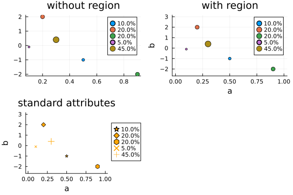
p5 = plot(d, dr; maxmarkersize = 20, title = "maxmarkersize 20")
p6 = plot(d, dr; minmarkersize = 4, title = "minmarkersize 4")
p7 = plot(d, dr; markersize = 5, title = "markersize 5")
p8 = plot(d, dr; label_formatter = (k, p, w) -> "$k: a = $(p[1])", title = "custom labels")
pb = plot(p5, p6, p7, p8)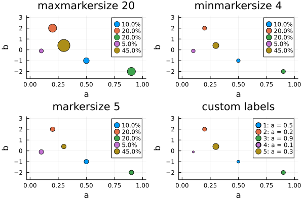
Since the design points are plotted in the given order, large points may be plotted over small ones. Unfortunately, the z-order of points can not be set independently in Plots.jl. Possible workarounds are sorting the points by decreasing weight before plotting, or choosing an unfilled marker shape.
d = DesignMeasure([0 1 1.01 2], [0.1, 0.1, 0.7, 0.1])
plot(d) # point at 1 not visible
plot(sort_weights(d; rev = true)) # point at 1 visible, but legend reordered
plot(d; markershape = :+) # all visible, but colors harder to distinguish
Kirstine.plot_gateauxderivative — Function
plot_gateauxderivative(d::DesignMeasure, adp::Kirstine.AbstractDesignProblem; <keyword arguments>)Plot the gateauxderivative in directions from a grid on region(adp), overlaid with the design points of d.
For 2-dimensional design regions, the default color gradient for the heat map is :diverging_bwr_55_98_c37_n256, which is perceptually uniform from blue via white to red. Custom gradients can be set via the fillcolor keyword argument. The standard plotting keyword arguments (markershape, markercolor, markersize, linecolor, linestyle, clims, ...) are supported. By default, markersize indicates the design weights.
Additional Keyword Arguments
n_grid::Union{Integer, Tuple{Integer}, Tuple{Integer, Integer}}: number of points in the grid. Must match the dimension of the design region. Defaults to101for one dimension, and to(51, 51)for two.overlay_points::Bool: draw alsopoints(d)on top of the graph. Defaults totrue.- Keyword arguments for plotting
DesignMeasures:label_formatter,minmarkersize,maxmarkersize. See the API reference for what they do.
Currently only implemented for 1- and 2-dimensional DesignRegions.
Kirstine.plot_expected_function — Function
plot_expected_function(
    f,
    g,
    h,
    xgrid::AbstractVector{<:Real},
    d::DesignMeasure,
    m::Kirstine.Model,
    cp::Kirstine.CovariateParameterization,
    pk::PriorSample;
    <keyword arguments>
)
Plot a graph of the pointwise expected value of a function and design points on that graph.
For user types C<:Kirstine.Covariate and p<:Kirstine.Parameter, the functions f, g, and h should have the following signatures:
f(x::Real, c::C, p::P)::Real. This function is for plotting a graph.g(c::C)::AbstractVector{<:Real}. This function is for plotting points, and should return the x coordinates corresponding toc.h(c::C, p::P)::AbstractVector{<:Real}. This function is for plotting points, and should return the y coordinates corresponding toc.
For each value of the covariate c implied by the design measure d, the following things will be plotted:
A graph of the average of
fwith respect topkas a function ofxevaluated at the elements ofxgrid. If differentcresult in identical graphs, only one will be plotted.Points at
g(c)andh(c, p)averaged with respect topk. By default, themarkersizeattribute is used to indicate the weight of the design point.
Additional Keyword Arguments
bands::Bool=false: plot pointwise credible bands. Currently only implemented for uniformweights(d). Color and opacity can be controlled with the standard keyword argumentsfillcolorandfillalpha.probability::Real=0.8: probability to use for the credible band.- Keyword arguments for plotting
DesignMeasures:label_formatter,minmarkersize,maxmarkersize. See the API reference for what they do.
Examples
For usage examples see the tutorial and dose-time-response vignettes.
source- YBT13Min Yang, Stefanie Biedermann, and Elina Tang (2013). On optimal designs for nonlinear models: a general and efficient algorithm. Journal of the American Statistical Association, 108(504), 1411–1420. doi:10.1080/01621459.2013.806268
- CK02Maurice Clerc and James Kennedy (2002). The particle swarm - explosion, stability, and convergence in a multidimensional complex space. IEEE Transactions on Evolutionary Computation, 6(1), 58–73. doi:10.1109/4235.985692
- ES00Russell C. Eberhardt and Yuhui Shi (2000). Comparing inertia weights and constriction factors in particle swarm optimization. Proceedings of the 2000 Congress on Evolutionary Computation. doi: 10.1109/CEC.2000.870279
- LJ15Simon Lacoste-Julien and Martin Jaggi (2015). On the Global Linear Convergence of Frank-Wolfe Optimization Variants. arXiv:1511.05932
- P23Sebastian Pokutta (2023). The Frank-Wolfe algorithm: a short introduction. Jahresbericht der Deutschen Mathematiker-Vereinigung, 126(1), 3–35. doi:10.1365/s13291-023-00275-x
- P06Friedrich Pukelsheim (2006). Optimal design of experiments. Wiley. doi:10.1137/1.9780898719109