Locally Optimal Design

This vignette briefly illustrates how to find a locally optimal design, and how to supply additional information to the solver when some design points or weights of the solution are already known.

While Kirstine.jl is primarily intended finding Bayesian optimal designs, finding locally optimal designs is also implicitly supported. For locally optimal design, one tries to maximize $\DesignCriterion(\TNIMatrix(\DesignMeasure, \Parameter_0))$ for some prior guess $\Parameter_0$. This prior guess can be thought of as a prior Dirac measure, making locally optimal design a special case of Bayesian optimal design.

Model Setup

For simplicity, we re-use the dose-response model from the tutorial.

using Kirstine, Random, Plots

@simple_model SigEmax dose
@simple_parameter SigEmax e0 emax ed50 h

function Kirstine.jacobianmatrix!(
    jm,
    m::SigEmaxModel,
    c::SigEmaxCovariate,
    p::SigEmaxParameter,
)
    dose_pow_h = c.dose^p.h
    ed50_pow_h = p.ed50^p.h
    A = dose_pow_h / (dose_pow_h + ed50_pow_h)
    B = ed50_pow_h * p.emax / (dose_pow_h + ed50_pow_h)
    jm[1, 1] = 1.0
    jm[1, 2] = A
    jm[1, 3] = -A * B * p.h / p.ed50
    jm[1, 4] = c.dose == 0 ? 0.0 : A * B * log(c.dose / p.ed50)
    return jm
end

Optimal Design

Instead of the sample from the multivariate normal distribution that we used in the introduction, we here only use its mean vector as the single guess for $\Parameter$.

guess = PriorSample([SigEmaxParameter(e0 = 1, emax = 2, ed50 = 0.4, h = 5)])
dp = DesignProblem(
    criterion = DCriterion(),
    region = DesignInterval(:dose => (0, 1)),
    model = SigEmaxModel(sigma = 1),
    covariate_parameterization = JustCopy(:dose),
    prior_knowledge = guess,
)

Locally optimal design problems are often simpler than fully Bayesian ones and can be solved with a smaller swarm and in fewer iterations.

str1 = DirectMaximization(
    optimizer = Pso(iterations = 50, swarmsize = 50),
    prototype = equidistant_design(region(dp), 4),
)

Random.seed!(31415)
s1, r1 = solve(dp, str1)
s1

DesignMeasure(
 [3.135435548592502e-5] => 0.25000767275725305,
 [0.3207541465365837] => 0.25003991892306177,
 [0.48364781547861957] => 0.24999249447251276,
 [1.0] => 0.24995991384717237,
)

gd = plot_gateauxderivative(s1, dp)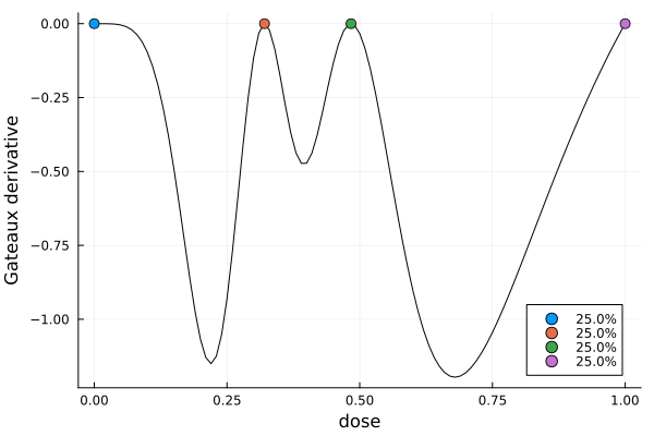

Keeping Points or Weights Fixed

Taking a closer look at s1, we notice two things:

1. The weights are nearly uniform.
2. The lowest and highest doses are at or near the boundaries of the design interval.

This is not by accident: one can show analytically^[LM07] that locally D-optimal designs for the sigmoid Emax model always have four design points with uniform weights, and that two of the points are at the minimal and maximal dose.

We can pass this information to the DirectMaximization strategy. The arguments fixedweights and fixedpoints take the indices of the weights (resp. doses) of the prototype that should not change during optimization. These weights and design points are also not randomized during the initialization of the swarm.

str2 = DirectMaximization(
    optimizer = Pso(iterations = 20, swarmsize = 50),
    prototype = equidistant_design(region(dp), 4),
    fixedweights = [1, 2, 3, 4],
    fixedpoints = [1, 4],
)

Random.seed!(31415)
s2, r2 = solve(dp, str2)
s2

DesignMeasure(
 [0.0] => 0.25,
 [0.32036023546981274] => 0.25,
 [0.48370009596035385] => 0.25,
 [1.0] => 0.25,
)