A Dose-Time-Response Model

This vignette covers four advanced topics:

• a two-dimensional^[2d] design region
• a non-trivial covariate parameterization
• vector units of observations
• the exchange algorithm

Note that although they are illustrated here together, any of them can also be used independently.

Our example model for this vignette will be a dose-time-response model. A dose-time-response model combines a pharmacokinetic (PK) model for a drug concentration that changes over time with a pharmacodynamic (PD) model that maps the concentration to a clinical outcome. The drug concentration itself is typically not observed. Specifically, we will combine a compartmental PK model with an Emax PD response. Optimal designs for this kind of model have been investigated for example by Fang and Hedayat^[FH08], Dette, Pepelyshev, and Wong^[DPW09], or Lange and Schmidli^[LS14].

Model Setup

In this section we implement the model in Julia. We defer the discussion of the design variables and the covariate parameterization to the following sections.

Concentration over time is governed by an absorption rate $a > 0$ and an elimination rate $e > 0$, where we assume $e < a$ for identifiability. Further, it depends on the initial dose $D$ administered at time $t=0$. The Emax response is parameterized by the baseline response $e_0$, the maximal effect above baseline $e_{\max{}}$, and the concentration of half-maximal effect $\mathrm{EC}_{50}$. The mean function $\MeanFunction$ is then obtained by combining these two.

\[\begin{aligned} c(t, a, e) &= \frac{D}{1-e/a}(\exp(-et) - \exp(-at)) \\ \mathrm{E}_{\max{}}(c, e_0, e_{\max{}}, \mathrm{EC}_{50}) &= e_0 + \frac{ce_{\max{}}}{\mathrm{EC}_{50} + c} \\ \MeanFunction((D, t_1,…,t_{\DimUnit}), θ) &= \begin{bmatrix} \mathrm{E}_{\max{}}(c(t_1, a, e), e_0, e_{\max{}}, \mathrm{EC}_{50})\\ … \\ \mathrm{E}_{\max{}}(c(t_{\DimUnit}, a, e), e_0, e_{\max{}}, \mathrm{EC}_{50})\\ \end{bmatrix} \end{aligned}\]

Hence the model covariates are the initial dose $D$ and the measurement times $t_1,…,t_{\DimUnit}$. In the following example, we will consider doses between 0 and 100 mg, and times between 0 and 24 hours. I.e. the covariate set is

\[\CovariateSet = [0, 100] × [0, 24]^{\DimUnit}.\]

A unit of observation is a vector $\Unit∈\Reals^{\DimUnit}$, collecting the responses at the $\DimUnit$ measurement times. The unknown model parameter is $\Parameter=(a, e, e_0, e_{\max{}}, \mathrm{EC}_{50})$.

For simplicity we assume that the measurements are uncorrelated with identical constant variances, i.e. $\UnitCovariance = σ^2 I_{\DimUnit}$. Since $σ$ enters the D-criterion objective only as a scaling factor, we may set $σ=1$ for the remainder of this text.

For this more complex model there are no helper macros and we have to implement not only the Jacobian matrix, but also the other necessary methods by hand.

using Kirstine, Random, Plots

@kwdef struct DTRMod <: Kirstine.NonlinearRegression
    sigma::Float64
    m::Int64
end

mutable struct DoseTimeCovariate <: Kirstine.Covariate
    dose::Float64
    time::Vector{Float64}
end

Kirstine.unit_length(m::DTRMod) = m.m
function Kirstine.update_model_vcov!(s, m::DTRMod, c::DoseTimeCovariate)
    fill!(s, 0.0)
    for j in 1:(m.m)
        s[j, j] = m.sigma^2
    end
end
Kirstine.allocate_covariate(m::DTRMod) = DoseTimeCovariate(0, zeros(m.m))

@simple_parameter DTR a e e0 emax ec50

function Kirstine.jacobianmatrix!(jm, m::DTRMod, c::DoseTimeCovariate, p::DTRParameter)
    for j in 1:length(c.time)
        A = exp(-p.a * c.time[j]) # calculate exponentials only once
        B = exp(-p.e * c.time[j])
        C = B - A
        rd = p.e - p.a # rate difference
        den = c.dose * C * p.a - rd * p.ec50
        den2 = den^2
        # ∂a
        jm[j, 1] = -c.dose * p.ec50 * p.emax * (A * c.time[j] * p.a * rd + p.e * C) / den2
        # ∂e
        jm[j, 2] = c.dose * p.a * p.ec50 * p.emax * (B * c.time[j] * rd + C) / den2
        # ∂e0
        jm[j, 3] = 1.0
        # ∂emax
        jm[j, 4] = c.dose * p.a * C / den
        # ∂ec50
        jm[j, 5] = c.dose * p.a * p.emax * C * rd / den2
    end
    return jm
end

Our example prior has an absorption rate that is about five times as large as the elimination rate, and the maximal concentration is reached after about 4 hours. The observable response varies between 1 and 3, with an $\mathrm{EC}_{50}$ at about 10.

function draw_from_prior(n)
    pars = map(
        0.5 .+ 0.10 .* randn(n),
        0.1 .+ 0.02 .* randn(n),
        1.0 .+ 0.25 .* randn(n),
        2.0 .+ 0.50 .* randn(n),
        exp.(2.3 .+ 0.6 .* randn(n)),
    ) do a, e, e0, emax, ec50
        return DTRParameter(a = a, e = e, e0 = e0, emax = emax, ec50 = ec50)
    end
    return PriorSample(pars)
end

The following is a small wrapper around plot_expected_function that plots a time-response curve for each initial dose and overlays the measurement point(s) implied by the design.

function plot_expected_response(d::DesignMeasure, dp::DesignProblem)
    response = function (D, t, p)
        con = D / (1 - p.e / p.a) * (exp(-p.e * t) - exp(-p.a * t))
        r = p.e0 + p.emax * con / (p.ec50 + con)
        return r
    end
    f(x, c, p) = response(c.dose, x, p)
    g(c) = c.time
    h(c, p) = [response(c.dose, t, p) for t in c.time]
    xrange = range(0, 24; length = 101)
    cp = covariate_parameterization(dp)
    plt = plot_expected_function(f, g, h, xrange, d, model(dp), cp, prior_knowledge(dp))
    plot!(plt; xguide = "time", yguide = "response", xticks = 0:4:24)
    return plt
end

Single Measurement

Let's start out really simple. Each patient will be measured exactly once. What are the optimal doses and dose-specific measurement times?

In terms of our model and the design problem this means

\[\begin{aligned} \DimUnit &= 1 \\ \DesignRegion &= [0, 100] × [0, 24] \\ \CovariateParameterization(\DesignPoint) &= (\DesignPoint_1, \DesignPoint_2) \\ \end{aligned}\]

i.e. the design region is identical to the covariate set.

struct CopyBoth <: Kirstine.CovariateParameterization end

function Kirstine.map_to_covariate!(c::DoseTimeCovariate, dp, m::DTRMod, cp::CopyBoth)
    c.dose = dp[1]
    c.time[1] = dp[2]
    return c
end

The next bit is new. In our dose-time-response model with the above covariate parameterization, design measures do not map injectively to information matrices. There are two reason for this:

1. With a dose $D=0$ the response is constantly $e_0$, no matter at which time we take measurements.
2. At time $t=0$ the response always starts at $e_0$, no matter what the initial dose was.

If we want unique design measures, we must implement a method for the simplify_unique function, which should choose a stable representative for a non-unique design measure. At the same time we should keep in mind numerical inaccuracies. One possibility is to

• set $D:=0$ if $t < ε_t$,
• and set $t:=0$ if $D < ε_D$

for some constants $ε_t ≥ 0$ and $ε_D ≥ 0$ that determine what counts as a “truly positive” time or dose.

Of course, we should only do this if $D=0$ and $t=0$ are in fact inside the design region.

function Kirstine.simplify_unique(
    d::DesignMeasure,
    dr::DesignInterval,
    m::DTRMod,
    cp::CopyBoth;
    minposdose = 0,
    minpostime = 0,
)
    res = deepcopy(d) # don't modify the input!
    if lowerbound(dr) == (0, 0)
        map(points(res)) do dp
            if dp[1] < minposdose || dp[2] < minpostime
                dp[1] = 0
                dp[2] = 0
            end
        end
    end
    return res
end

The next steps are as in the tutorial: set up the design problem and solve it with direct maximization.

Random.seed!(4711)
dp1 = DesignProblem(
    criterion = DCriterion(),
    region = DesignInterval(:dose => (0, 100), :time => (0, 24)),
    model = DTRMod(sigma = 1, m = 1),
    covariate_parameterization = CopyBoth(),
    prior_knowledge = draw_from_prior(1000),
)

Random.seed!(1357)
st1 = DirectMaximization(
    optimizer = Pso(swarmsize = 30, iterations = 100),
    prototype = random_design(region(dp1), 7),
)

Random.seed!(2468)
s1, r1 = solve(dp1, st1; minpostime = 1e-3, minposdose = 1e-3, maxdist = 1e-2)
s1

DesignMeasure(
 [0.0, 0.0] => 0.20053030795126034,
 [14.310132703488692, 7.9551274923954916] => 0.19811209094488025,
 [61.493484624092964, 24.0] => 0.07683680630261554,
 [99.99929278721805, 4.0783147418405] => 0.1974719271387898,
 [100.0, 0.1730851666925906] => 0.19894174306143625,
 [100.0, 23.998585546217786] => 0.12810712460101797,
)

To sort the design point by time instead of dose, we can use the dimorder argument of sort_points. We could also have directly passed it to solve.

sort_points(s1; dimorder = [2, 1])

DesignMeasure(
 [0.0, 0.0] => 0.20053030795126034,
 [100.0, 0.1730851666925906] => 0.19894174306143625,
 [99.99929278721805, 4.0783147418405] => 0.1974719271387898,
 [14.310132703488692, 7.9551274923954916] => 0.19811209094488025,
 [100.0, 23.998585546217786] => 0.12810712460101797,
 [61.493484624092964, 24.0] => 0.07683680630261554,
)

For a two-dimensional design region, the gateaux derivative is plotted as a heatmap.

gd1 = plot_gateauxderivative(s1, dp1)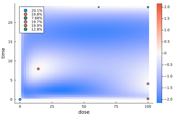

The next plot shows the expected time-response curve for the dose of each design point. Additionally the measurement times themselves are indicated on their respective curves.

er1 = plot_expected_response(s1, dp1)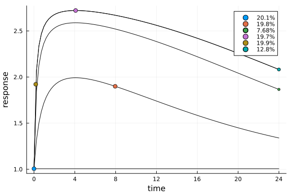

Optimal Time

Next, let's consider a variant of the previous design problem that was investigated by Fang and Hedayat^[FH08]. They were only interested in a single optimal measurement time for each patient, while taking the initial dose $D$ as given and fixed.

\[\begin{aligned} m &= 1 \\ \DesignRegion &= [0, 24] \\ \CovariateParameterization(\DesignPoint) &= (D, \DesignPoint) \end{aligned}\]

This time there are no problems with uniqueness and the implementation is straightforward. Note how the DesignProblem differs from dp1 only in its design region and its covariate parameterization.

struct FixedDose <: Kirstine.CovariateParameterization
    dose::Float64
end

function Kirstine.map_to_covariate!(c::DoseTimeCovariate, dp, m::DTRMod, cp::FixedDose)
    c.dose = cp.dose
    c.time[1] = dp[1]
    return c
end

dp2 = DesignProblem(
    dp1;
    region = DesignInterval(:time => (0, 24)),
    covariate_parameterization = FixedDose(100),
)

Random.seed!(111317)
st2 = DirectMaximization(
    optimizer = Pso(swarmsize = 30, iterations = 50),
    prototype = random_design(region(dp2), 5),
)

Random.seed!(14916)
s2, r2 = solve(dp2, st2)
s2

DesignMeasure(
 [0.0] => 0.1996347804123737,
 [0.15441476713296678] => 0.2000666280210823,
 [2.2462632650730114] => 0.20067467321750976,
 [13.338793671645664] => 0.19962045785683455,
 [24.0] => 0.2000034604921996,
)

gd2 = plot_gateauxderivative(s2, dp2)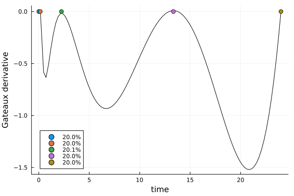

er2 = plot_expected_response(s2, dp2)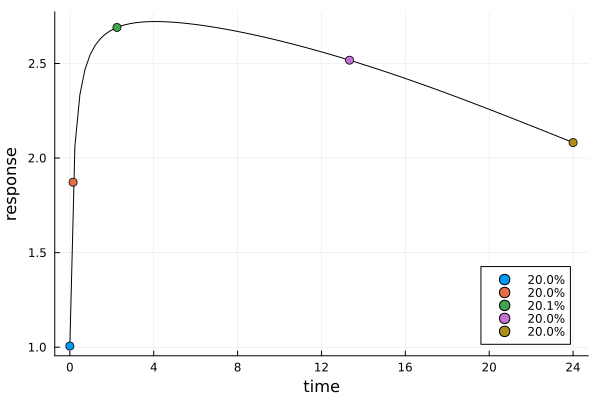

Optimal Dose

In this section we consider kind of the opposite of the previous problem. Lange and Schmidli^[LS14] considered a fixed number of measurements per patient at regular intervals, and were interested in optimal initial doses only.

\[\begin{aligned} m &= 13 \\ \DesignRegion &= [0, 100] \\ \CovariateParameterization(\DesignPoint) &= (\DesignPoint, 0, 2, …, 24) \\ \end{aligned}\]

struct FixedTimes <: Kirstine.CovariateParameterization
    time::Vector{Float64}
end

function Kirstine.map_to_covariate!(c::DoseTimeCovariate, dp, m::DTRMod, cp::FixedTimes)
    c.dose = dp[1]
    c.time .= cp.time
    return c
end

dp3 = DesignProblem(
    dp1;
    region = DesignInterval(:dose => (0, 100)),
    model = DTRMod(1, 13), # measurements every two hours
    covariate_parameterization = FixedTimes(0:2:24),
)

Random.seed!(9630)
st3 = DirectMaximization(
    optimizer = Pso(swarmsize = 25, iterations = 20),
    prototype = equidistant_design(region(dp3), 5),
)

Random.seed!(1827)
s3, r3 = solve(dp3, st3; maxweight = 1e-4)
s3

DesignMeasure(
 [0.0] => 0.1051865637147946,
 [15.949800420851398] => 0.4847347290784628,
 [100.0] => 0.41007870720674255,
)

gd3 = plot_gateauxderivative(s3, dp3)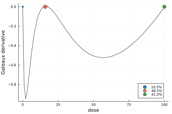

Each design point now corresponds to 13 individual measurements.

er3 = plot_expected_response(s3, dp3)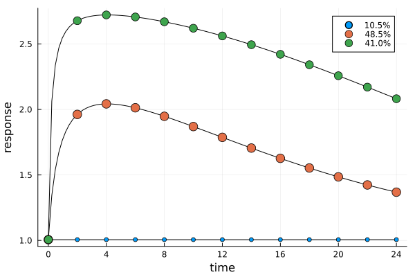

Equidistant Times

Next, let's say we want to keep measuring each patient 13 times at regular intervals. But maybe we can do better than using the same interval regardless of the dose. Let's try to find dose-specific optimal $Δt$ between measurements! To keep the results comparable, we allow $Δt∈[0, 2]$, resulting in a latest measurement time at 24 hours.

\[\begin{aligned} m &= 13 \\ \DesignRegion &= [0, 100] × [0, 2] \\ \CovariateParameterization(z) &= (z_1, 0, z_2, 2z_2, …, 12z_2)\\ \end{aligned}\]

For this setup we need to think about uniqueness again.

• With $Δt=0$ we would measure 13 times at $t=0$, which is not sensible in context. But since the same response is obtained with $D=0$ and arbitrary $Δt$, we set such a design point to $(0, 2)$.

• Similarly, with $D=0$ the response is constantly $e_0$. Here we also set the design point to $(0, 2)$.

struct EquidistantTimes <: Kirstine.CovariateParameterization end

function Kirstine.map_to_covariate!(
    c::DoseTimeCovariate,
    dp,
    m::DTRMod,
    cp::EquidistantTimes,
)
    c.dose = dp[1]
    for i in 1:(m.m)
        c.time[i] = (i - 1) * dp[2]
    end
    return c
end

function Kirstine.simplify_unique(
    d::DesignMeasure,
    dr::DesignInterval,
    m::DTRMod,
    cp::EquidistantTimes;
    minposdose = 0,
    minposdelta = 0,
)
    res = deepcopy(d)
    if lowerbound(dr)[1] == 0
        map(points(res)) do dp
            if dp[1] <= minposdose
                dp[1] = 0
                dp[2] = upperbound(dr)[2]
            end
        end
        if lowerbound(dr)[2] == 0
            map(points(res)) do dp
                if dp[2] <= minposdelta
                    dp[1] = 0
                    dp[2] = upperbound(dr)[2]
                end
            end
        end
    end
    return res
end

dp4 = DesignProblem(
    dp3;
    region = DesignInterval(:dose => (0, 100), :Δt => (0, 2)),
    covariate_parameterization = EquidistantTimes(),
)

Random.seed!(124816)
st4a = DirectMaximization(
    optimizer = Pso(swarmsize = 25, iterations = 75),
    prototype = random_design(region(dp4), 5),
)

Random.seed!(112358)
s4a, r4a = solve(dp4, st4a; minposdose = 1e-3)
gd4a = plot_gateauxderivative(s4a, dp4; legend = :bottomleft)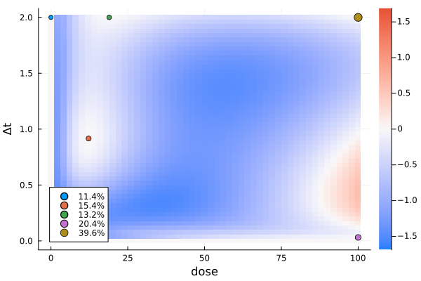

This does not look like the solution yet. There are several things that could have happened.

• The particle swarm optimizer was not run for enough iterations.

• The optimizer got stuck in a local maximum, possibly because the number of design points is too small.

pr4a = plot(r4a)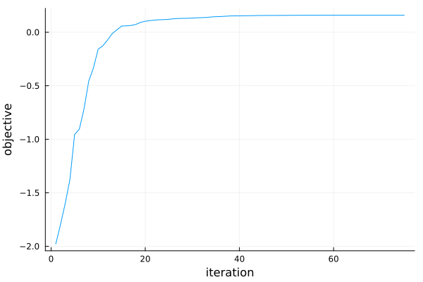

Looking at the optimization progress it seems that running with more iterations will not help.

We could try direct maximization again, this time with a prototype with more design points. But there is a smarter thing we can try instead. The Exchange algorithm can be understood as a kind of coordinate-wise infinite-dimensional gradient ascent, since it basically alternates the following two actions

1. Find the point $\DesignPoint ∈ \DesignRegion$ where the corresponding Gateaux derivative is largest and add it to the design measure.

2. Re-optimize only the weights, then drop any points with zero weight.

Running this with a random starting design can be slow to converge, but since we already have promising candidate, we can hope that it gives us the solution after a few steps.

For part 1, we will not use PSO, but a Kirstine.GridSearch over the design region $\DesignRegion$. This has the advantage that grid search is deterministic and will always find the maximum (on the grid), while Pso may sometimes get stuck in a local maximum and make the overall exchange algorithm somewhat unstable. On the other hand, grid search on a very fine grid can take a lot of time.

In this particular example we save some runtime since we can reasonably guess that a single step of the exchange algorithm might be sufficient, and that the new point will be added at a point with $D=100$. This is why we can get away with a Kirstine.ProductGrid that has only 2 different dose values. For the second dimension, the grid has 51 different values at $Δt=0,0.04,…,2$.

st4b = Exchange(
    candidate = s4a,
    steps = 1,
    optimizer_direction = Kirstine.GridSearch(gridspec = Kirstine.ProductGrid(2, 51)),
    optimizer_weight = Pso(swarmsize = 25, iterations = 50),
)

Random.seed!(314)
s4b, r4b = solve(dp4, st4b; minposdose = 1e-3, maxdist = 2e-2)

Let's look at the solution.

s4b

DesignMeasure(
 [0.0, 2.0] => 0.11343676907254417,
 [12.258680316012303, 0.9158234222042569] => 0.1466543099306418,
 [18.960755545027716, 2.0] => 0.1450562405792781,
 [99.99958420409529, 0.030724171006199445] => 0.19609399574206807,
 [100.0, 0.44] => 0.051532056457751135,
 [100.0, 2.0] => 0.34722662821771666,
)

efficiency(s4a, s4b, dp4)

0.9969896414364555

gd4b = plot_gateauxderivative(s4b, dp4; legend = :bottomleft)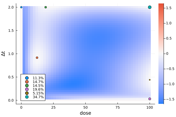

er4 = plot_expected_response(s4b, dp4)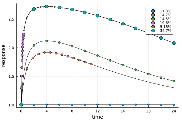

Log-Equidistant Times

Finally, let's consider a variant of the previous problem, but this time with equidistant measurement times on the log scale. For some multiplier $b>1$ we have:

\[\begin{aligned} m &= 13 \\ \DesignRegion &= [0, 100] × [0, 24/b^{\DimUnit-2}] \\ \CovariateParameterization(z) &= (z_1, 0, z_2, bz_2, b^2z_2, …, b^{\DimUnit-2}z_2)\\ \end{aligned}\]

In the following example we take $b=\sqrt{2}$.

struct LogEquidistantTimes <: Kirstine.CovariateParameterization
    b::Float64
end

function Kirstine.map_to_covariate!(
    c::DoseTimeCovariate,
    dp,
    m::DTRMod,
    cp::LogEquidistantTimes,
)
    if m.m < 2
        error("need at least 2 measurements for LogEquidistantTimes")
    end
    c.dose = dp[1]
    c.time[1] = 0
    c.time[2] = dp[2]
    for j in 3:(m.m)
        c.time[j] = cp.b * c.time[j - 1]
    end
    return c
end

function Kirstine.simplify_unique(
    d::DesignMeasure,
    dr::DesignInterval,
    m::DTRMod,
    cp::LogEquidistantTimes;
    minposdose = 0,
    minposdelta = 0,
)
    res = deepcopy(d)
    if lowerbound(dr)[1] == 0
        map(points(res)) do dp
            if dp[1] <= minposdose
                dp[1] = 0
                dp[2] = upperbound(dr)[2]
            end
        end
        if lowerbound(dr)[2] == 0
            map(points(res)) do dp
                if dp[2] <= minposdelta
                    dp[1] = 0
                    dp[2] = upperbound(dr)[2]
                end
            end
        end
    end
    return res
end

dp5 = DesignProblem(
    dp3;
    covariate_parameterization = LogEquidistantTimes(sqrt(2)),
    region = DesignInterval(:dose => (0, 100), :Δt => (0, 24 / 45.25483399593908)),
)

Random.seed!(132435)
st5 = DirectMaximization(
    optimizer = Pso(swarmsize = 40, iterations = 80),
    prototype = random_design(region(dp5), 5),
)

Random.seed!(6283)
s5, r5 = solve(dp5, st5; maxdist = 1e-3, maxweight = 1e-3, minposdelta = 1e-3)
s5

DesignMeasure(
 [0.0, 0.5303300858899102] => 0.10958860244868715,
 [17.56761395230221, 0.5303275816838873] => 0.3992041718670002,
 [99.99726947723131, 0.011673829992532737] => 0.05224177785883233,
 [100.0, 0.5303300122682958] => 0.43896544782548025,
)

gd5 = plot_gateauxderivative(s5, dp5; legend = :bottomleft)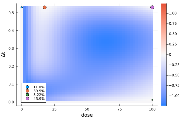

er5 = plot_expected_response(s5, dp5)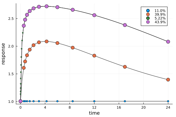

Efficiency Comparison

Let's finally compare the relative efficiency of all these designs under their respective design problems:

sol_prob = Iterators.zip([s1, s2, s3, s4b, s5], [dp1, dp2, dp3, dp4, dp5])
eff = [efficiency(d1, d2, p1, p2) for (d1, p1) in sol_prob, (d2, p2) in sol_prob]

5×5 Matrix{Float64}:
  1.0        1.48507  0.126509   0.0930306  0.101641
  0.673371   1.0      0.0851876  0.0626441  0.0684424
  7.90457   11.7388   1.0        0.735367   0.803431
 10.7491    15.9632   1.35987    1.0        1.09256
  9.83851   14.6108   1.24466    0.915283   1.0

In this matrix, d1 varies over rows and d2 varies over columns. We see that s1 is better than s2 (not surprising, since the former can have time-specific doses), and that s3 through s5 are better than both s1 and s2. We further see that both s4b and s5 are better than s3 (again not surprising, since the former has dose-specific intervals), and that s4b is slightly better than s5.

But in a sense this comparison is not entirely fair. What we have computed above is the efficiency in terms of units of observation. But isn't a unit with 13 measurements already inherently “larger” than a unit with only 1? Because of our choice of $\UnitCovariance$, a different comparison can be devised. Since we assumed uncorrelated within-unit errors with $\UnitCovariance = σ^2I_{\DimUnit}$ any of the solutions s2 through s5 can be identified with a candidate solution for dp1. For example, we can “split up” a design point from s4,

\[(D, Δt),\]

into $\DimUnit$ separate design points

\[(D, 0), (D, Δt), (D, 2Δt), …, (D, (\DimUnit - 1)Δt),\]

each with $1/\DimUnit$ the original weight.

Framed like that, it can make sense to compare efficiency in terms of single measurements. To compute this, we need to multiply eff by the inverse ratio of unit lengths for the designs under comparison, i.e.

\[\frac{\DimUnit^{(2)}}{\DimUnit^{(1)}} \RelEff(\DesignMeasure_1, \DesignMeasure_2).\]

eff .* [1 1 13 13 13] ./ [1, 1, 13, 13, 13]

5×5 Matrix{Float64}:
 1.0       1.48507   1.64462  1.2094    1.32134
 0.673371  1.0       1.10744  0.814374  0.889751
 0.608044  0.902985  1.0      0.735367  0.803431
 0.826858  1.22794   1.35987  1.0       1.09256
 0.756809  1.12391   1.24466  0.915283  1.0

Now we see that no design is better than s1. This is not surprising, since any of the solutions for dp2 through dp5 can be identified with a candidate solution for dp1, but d1 is already optimal for dp1.