New Normal Approximation
Locally optimal designs for a transformation of the model parameter often don't exist, since they correspond to singular information matrices where the objective function is undefined or negative infinity [fn1]. Faced with this problem, some authors resort to ad-hoc matrix regularization, i.e. they add a small symmetric positive definite matrix $R$ to the singular average Fisher information matrix:
\[\NIMatrix^{\text{reg}}(\DesignMeasure, \Parameter) = \AverageFisherMatrix(\DesignMeasure, \Parameter) + R.\]
While this approach fixes the problem of undefined objective functions, it creates several new problems with the interpretation of the results.
From a Bayesian perspective, the regularized matrix above can be thought of as arising from a regression model in which $\Parameter$ has a multivariate normal prior with covariance matrix
\[\Covariance(\Parameter) = \SampleSize R^{-1}.\]
That's problematic because now the information in the prior scales with sample size; i.e., the prior's influence does not vanish when $n → ∞$. Additionally, since locally optimal design is formally equivalent to design with a degenerate $\DiracDist(\Parameter_0)$ prior, the whole setup is inconsistent since this prior has zero covariance.
With $\NIMatrix^{\text{reg}}$ we also can't to compute a proper relative efficiency, since we can't pull the sample sizes $\SampleSize^{(1)}$ and $\SampleSize^{(2)}$ out of the determinant. While we still can compute the expression
\[\exp\biggl( \frac{1}{\DimTransformedParameter} \IntD{\ParameterSet}{ \log\frac{\det \TNIMatrix^{\text{reg}}(\DesignMeasure_1, \Parameter)}{\det \TNIMatrix^{\text{reg}}(\DesignMeasure_2, \Parameter)} }{\PriorDensity(\Parameter)}{\Parameter} \biggr)\]
it does not correspond to a ratio of sample sizes anymore.
With these warnings out of the way, let's look at the implementation.
Implementation
We define a new subtype of Kirstine.NormalApproximation and a corresponding method for the internal informationmatrix! function. In its first argument it receives the average Fisher information matrix which it should overwrite with the normalized information matrix.
using Kirstine, Plots, Random
using LinearAlgebra: diagm, rank, cond

struct RegularizedFisherMatrix <: Kirstine.NormalApproximation
    R::Matrix{Float64}
end

function Kirstine.informationmatrix!(
    afm::AbstractMatrix{<:Real},
    na::RegularizedFisherMatrix,
)
    afm .+= na.R
    return afm
end
Example
As an example we compute a locally optimal design for estimating the time to maximum concentration in Atkinson et al.'s compartmental model.
We compare this to the design for estimating all of $\Parameter$, both for the unregularized and the regularized information matrix. Note that we use 1e-4 as the diagonal elements of R, whereas the original publication uses 1e-5. The smaller amount of regularization does not seem to be sufficient for producing numerically stable results.
@simple_model TPC time
@simple_parameter TPC a e s

function Kirstine.jacobianmatrix!(jm, m::TPCModel, c::TPCCovariate, p::TPCParameter)
    A = exp(-p.a * c.time)
    E = exp(-p.e * c.time)
    jm[1, 1] = A * p.s * c.time
    jm[1, 2] = -E * p.s * c.time
    jm[1, 3] = E - A
    return m
end

function Dttm(p)
    A = p.a - p.e
    A2 = A^2
    B = log(p.a / p.e)
    da = (A / p.a - B) / A2
    de = (B - A / p.e) / A2
    ds = 0
    return [da de ds]
end

dp_i = DesignProblem(
    region = DesignInterval(:time => [0, 48]),
    criterion = DCriterion(),
    covariate_parameterization = CopyTo(:time),
    model = TPCModel(sigma = 1),
    prior_knowledge = PriorSample([TPCParameter(a = 4.298, e = 0.05884, s = 21.80)]),
    transformation = Identity(),
    normal_approximation = FisherMatrix(),
)

rfm_em4 = RegularizedFisherMatrix(diagm(fill(1e-4, 3)))
dp_ir = DesignProblem(dp_i; normal_approximation = rfm_em4)
dp_tr = DesignProblem(dp_ir; transformation = DeltaMethod(Dttm))

strategy = DirectMaximization(
    optimizer = Pso(swarmsize = 100, iterations = 50),
    prototype = uniform_design([[0], [24], [48]]),
)

problems = [dp_ir, dp_i, dp_tr]

(s_ir, r_ir), (s_i, r_i), (s_tr, r_tr) = map(problems) do dp
    Random.seed!(1357)
    solve(dp, strategy; maxweight = 1e-3, maxdist = 1e-2)
end

gds = map([s_ir, s_i, s_tr], problems, ["id reg", "id unreg", "ttm reg"]) do s, dp, title
    plot_gateauxderivative(s, dp; title = title)
end

gd = plot(gds...)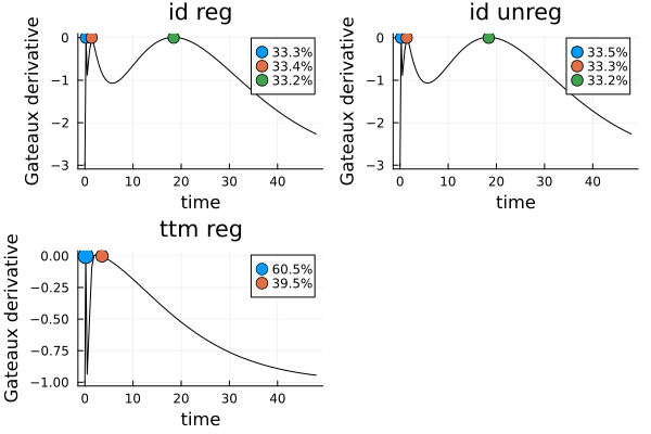
As we can see, the two solutions for the Identity transformation are essentially equal, and the solution for time-to-maximum-concentration has only two design points.
s_iDesignMeasure(
[0.23013409526910428] => 0.33511278577983994,
[1.382677276250709] => 0.3327747503342542,
[18.406782431481943] => 0.3321124638859059,
)s_irDesignMeasure(
[0.22952215512284513] => 0.33344530357348345,
[1.3871489127809553] => 0.3341689660845956,
[18.43237368022909] => 0.33238573034192087,
)s_trDesignMeasure(
[0.18009461306034247] => 0.6051847764968658,
[3.561491759806154] => 0.39481522350313425,
)As expected, s_tr is singular when no regularization is employed:
dp_t = DesignProblem(dp_i; transformation = DeltaMethod(Dttm))
objective(s_tr, dp_t)-InfThis is also reflected in the rank of the information matrix:
function infomat(d::DesignMeasure, dp::DesignProblem)
    Kirstine.informationmatrix(
        d,
        model(dp),
        covariate_parameterization(dp),
        parameters(prior_knowledge(dp))[1],
        normal_approximation(dp),
    )
end
(rank(infomat(s_tr, dp_t)), rank(infomat(s_tr, dp_tr)))
(2, 3)Regularization brings down the condition number from "abysmal" to merely "not great":
cond(infomat(s_tr, dp_t)), cond(infomat(s_tr, dp_tr))(7.249291374775448e18, 1.5745668441886386e7)Compare this to the Bayesian optimal design for the proper prior distribution, which naturally has three points and is nonsingular. We evaluate it with the objective for unregularized locally optimal design:
bopt = DesignMeasure(
    [0.1785277717204147] => 0.6022152518991615,
    [2.4347788334799083] => 0.2985274392389716,
    [8.778030603264321] => 0.09925730886186684,
)
objective(bopt, dp_t)3.560915425578755It implies similar condition numbers as s_i and s_ir.
cond(infomat(bopt, dp_t)),
cond(infomat(bopt, dp_tr)),
cond(infomat(s_i, dp_i)),
cond(infomat(s_ir, dp_ir))
(26496.637989885166, 26460.39471836411, 33505.61669151681, 33374.01990153766)The Gateaux derivative of the locally optimal design with two points is also rather sensitive to perturbations, while for all the designs with three points it is not:
function perturb_points(d::DesignMeasure, fac::Real)
    return DesignMeasure(reduce(hcat, points(d)) .* fac, deepcopy(weights(d)))
end

gds_perturbed = [
    plot_gateauxderivative(perturb_points(s_ir, 1.001), dp_ir; title = "id reg")
    plot_gateauxderivative(perturb_points(s_i, 1.001), dp_i; title = "id unreg")
    plot_gateauxderivative(perturb_points(s_tr, 1.001), dp_tr; title = "ttm reg")
    plot_gateauxderivative(perturb_points(bopt, 1.001), dp_t; title = "ttm unreg Bayes")
]
gdp = plot(gds_perturbed...)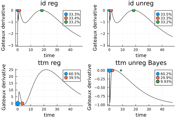
- fn1Bayesian optimal designs do not have this problem, since a proper prior always provides some information on all model parameters, even when the data do not.