A Simple Dose-Response Model
This vignette describes how to set up a simple nonlinear regression model in order to find a Bayesian D-optimal design for estimating the model parameter.
Model
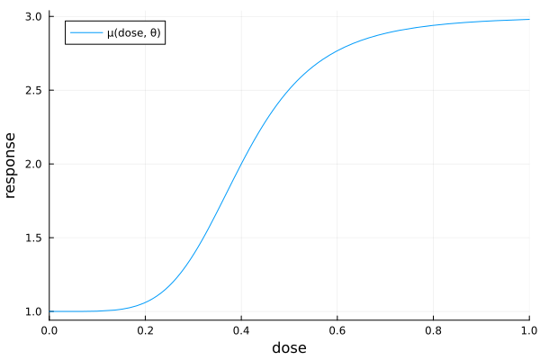
Suppose we want to investigate the dose-response relationship between a drug and some clinical outcome. A commonly used model for this task is the sigmoid Emax model: an s-shaped curve with four parameters. Assuming independent measurement errors, the corresponding regression model for a total of $\SampleSize$ observations at $\NumDesignPoints$ different dose levels $\Covariate_1,\dots,\Covariate_{\IndexDesignPoint}$ is
\[\Unit_{\IndexUnit} \mid \Parameter \overset{\mathrm{iid}}{\sim} \mathrm{Normal}(\MeanFunction(\Covariate_{\IndexDesignPoint}, \Parameter), \sigma^2) \quad \text{for all } \IndexUnit \in I_{\IndexDesignPoint}, \IndexDesignPoint = 1, \dots, \NumDesignPoints,\]
with expected response at dose $\Covariate$
\[\MeanFunction(\Covariate, \Parameter) = E_0 + E_{\max{}} \frac{\Covariate^h}{\mathrm{ED}_{50}^h + \Covariate^h}\]
and a four-element parameter vector $\Parameter = (E_0, E_{\max{}}, \mathrm{ED}_{50}, h)$. Here, $E_0$ is the baseline response, $E_{\max{}}$ is the maximum effect above (or below) baseline, $\mathrm{ED}_{50} > 0$ is the dose at which half of the maximum effect is attained, and $h > 0$ controls the steepness of the increasing (or decreasing) part of the curve.
using Plots
θ = (e0 = 1, emax = 2, ed50 = 0.4, h = 5)
pse = plot(
    x -> θ.e0 + θ.emax * x^θ.h / (θ.ed50^θ.h + x^θ.h);
    xlims = (0, 1),
    xguide = "dose",
    yguide = "response",
    label = "μ(dose, θ)",
)
In order to find an optimal design, we need to know the Jacobian matrix of $\MeanFunction(\Covariate, \Parameter)$ with respect to $\Parameter$. Calculating manually, or using a computer algebra system such as Maxima or WolframAlpha, we find
\[\begin{aligned} \partial_{E_0} \MeanFunction(\Covariate, \Parameter) &= 1 \\ \partial_{E_{\max{}}} \MeanFunction(\Covariate, \Parameter) &= \frac{\Covariate^h}{\mathrm{ED}_{50}^h + \Covariate^h}\\ \partial_{\mathrm{ED}_{50}} \MeanFunction(\Covariate, \Parameter) &= \frac{h E_{\max{}} \Covariate^h\mathrm{ED}_{50}^{h-1}}{(\mathrm{ED}_{50}^h + \Covariate^h)^2} \\ \partial_{h} \MeanFunction(\Covariate, \Parameter) &= \frac{E_{\max{}} \Covariate^h \mathrm{ED}_{50}^h (\log(\Covariate / \mathrm{ED}_{50}))}{(\mathrm{ED}_{50}^h + \Covariate^h)^2} \\ \end{aligned}\]
for $\Covariate \neq 0$, and the limit
\[\lim_{\Covariate\to0} \partial_{h} \MeanFunction(\Covariate, \Parameter) = 0.\]
Setup
For specifying a model and a design problem, Kirstine.jl makes use of Julia's extendable type system and method dispatching. If your working knowledge of this is rusty, now would be a good time to refresh it.
Model and Design Region
In Kirstine.jl, the regression model is defined by subtyping Kirstine.NonlinearRegression, Kirstine.Covariate, Kirstine.Parameter, and Kirstine.CovariateParameterization, and implementing a handful of methods for them.
In the sigmoid Emax model, a single unit of observation is just a real number $\Unit_{\IndexUnit}$. For such a case, we can use the helper macro @simple_model to declare a model type named SigEmaxModel, and a covariate type named SigEmaxCovariate with the single field dose.
using Kirstine
@simple_model SigEmax dose
The model parameter $\Parameter$ is just a vector with no additional structure, which is why we can use the helper macro @simple_parameter to define a parameter type SigEmaxParameter with the Float64 fields e0, emax, ed50, and h.
@simple_parameter SigEmax e0 emax ed50 h(The @simple_model and @simple_parameter macros also set up methods for a few helper functions that dispatch on these newly defined types. The details are in the macros' docstrings and the api docs. They are not relevant for this tutorial, but you should look them up when you need to implement a more complex model, like the one in the dose-dime-response example.)
Next we implement the Jacobian matrix. We do this by defining a method for Kirstine.jacobianmatrix! that specializes on our newly defined model, covariate and parameter types. This method will later be called from the package internals with a preallocated matrix jm (of size (1, 4)). Now our job is to fill in the correct values:
function Kirstine.jacobianmatrix!(
    jm,
    m::SigEmaxModel,
    c::SigEmaxCovariate,
    p::SigEmaxParameter,
)
    dose_pow_h = c.dose^p.h
    ed50_pow_h = p.ed50^p.h
    A = dose_pow_h / (dose_pow_h + ed50_pow_h)
    B = ed50_pow_h * p.emax / (dose_pow_h + ed50_pow_h)
    jm[1, 1] = 1.0
    jm[1, 2] = A
    jm[1, 3] = -A * B * p.h / p.ed50
    jm[1, 4] = c.dose == 0 ? 0.0 : A * B * log(c.dose / p.ed50)
    return jm
end
Note that for defining the design problem we do not need to implement the mean function $\MeanFunction$ itself, but only its Jacobian matrix $\TotalDiff\MeanFunction$ with respect to $\Parameter$.
The jacobianmatrix! function is the main place for achieving efficiency gains. Note how we have rearranged the derivatives such that we compute the expensive exponentials only once. (We also follow the conventions and also return the modified argument jm.)
Next, we set up the design region. Let's say we want to allow doses between 0 and 1 (in some unit).
dr = DesignInterval(:dose => (0, 1))A design will then be a discrete probability measure with atoms (design points) from dr, and a design point is represented by a Vector{Float64}. In our simple model, these vectors have length 1.
Finally, we need to specify how a design point maps to a SigEmaxCovariate. Here, the design region is simply the interval of possible doses. This means that we can just copy the only element of the design point into the covariate's dose field. For this we can use CopyTo, which is a subtype of Kirstine.CovariateParameterization.
cp = CopyTo(:dose)Prior Knowledge
For Bayesian optimal design of experiments we need to specify a prior distribution on $\Parameter$. Kirstine.jl then needs a sample from this distribution.
For this example we use independent normal priors on the elements of $\Parameter$. We first draw a vector of SigEmaxParameter values which we then wrap into a PriorSample.
using Random
Random.seed!(31415)

theta_mean = [1, 2, 0.4, 5]
theta_sd = [0.5, 0.5, 0.05, 0.5]
sep_draws = map(1:1000) do i
    rnd = theta_mean .+ theta_sd .* randn(4)
    return SigEmaxParameter(e0 = rnd[1], emax = rnd[2], ed50 = rnd[3], h = rnd[4])
end
prior_sample = PriorSample(sep_draws)
Note that the SigEmaxParameter constructor takes keyword arguments.
Design Problem
Now we collect all the parts in a DesignProblem.
dp = DesignProblem(
    criterion = DCriterion(),
    region = dr,
    model = SigEmaxModel(sigma = 1),
    covariate_parameterization = cp,
    prior_knowledge = prior_sample,
)
Note that the SigEmaxModel constructor takes the measurement standard deviation $σ$ as an argument. For D-optimality, this only scales the objective function and has no influence on the optimal design. This is why we simply set it to 1 here.
Optimal Design
Kirstine.jl provides several high-level Kirstine.ProblemSolvingStrategy types for solving the design problem dp. A very simple, but often quite effective one, is direct maximization with a particle swarm optimizer.
Apart from the Pso parameters, the DirectMaximization strategy needs to know how many points the design measures should have. This is indirectly specified by the prototype argument: it takes a DesignMeasure which is then used for initializing the swarm. One particle is set exactly to prototype. The remaining ones have the same number of design points, but their weights and design points are completely randomized. For our example, we use a prototype with 8 equally spaced design points.
strategy = DirectMaximization(
    optimizer = Pso(iterations = 50, swarmsize = 100),
    prototype = equidistant_design(dr, 8),
)

Random.seed!(54321)
s1, r1 = solve(dp, strategy)
The solve function returns two objects:
s1: a slightly postprocessedDesignMeasurer1: aKirstine.DirectMaximizationResultthat contains diagnostic information about the optimization run.
We can access the lower-level Kirstine.OptimizationResult by calling optimization_result on r1, which will show some statistics when printed:
optimization_result(r1)OptimizationResult
* iterations: 50
* objective evaluations: 5000
* gradient evaluations: 0
* elapsed time: 0:00:07.592
* converged: false
* traced states: 0
* state type: Kirstine.PsoState{DesignMeasure, Kirstine.SignedMeasure}
* maximum: -6.7206347777662705
* maximizer: DesignMeasure(
[0.0] => 0.13404889547477042,
[0.28680117509990044] => 0.1385323232912528,
[0.35590085349128153] => 0.024903749604217627,
[0.3567666844285769] => 0.12742156052917672,
[0.49982025315652223] => 0.22264826193961815,
[0.010691842729708925] => 0.1077006446024656,
[1.0] => 0.1259454888888293,
[1.0] => 0.11879907566966932,
)The solution s1 is displayed as designpoint => weight pairs.
s1DesignMeasure(
[0.0] => 0.13404889547477042,
[0.010691842729708925] => 0.1077006446024656,
[0.28680117509990044] => 0.1385323232912528,
[0.35590085349128153] => 0.024903749604217627,
[0.3567666844285769] => 0.12742156052917672,
[0.49982025315652223] => 0.22264826193961815,
[1.0] => 0.24474456455849863,
)Looking closely at s1, we notice that two design points are nearly identical:
[0.35590085349128153] => 0.024903749604217627
[0.3567666844285769] => 0.12742156052917672
It seems plausible that they would merge to a single one if we ran the optimizer for some more iterations. But we can also do this after the fact by calling simplify on the solution. This way we merge all design points that are less than some maximum distance apart, and remove all design points with negligible weight.
s2 = sort_points(simplify(s1, dp, maxweight = 1e-3, maxdist = 2e-2))DesignMeasure(
[0.004763270091889071] => 0.24174954007723604,
[0.28680117509990044] => 0.1385323232912528,
[0.3566251292474773] => 0.15232531013339434,
[0.49982025315652223] => 0.22264826193961815,
[1.0] => 0.24474456455849863,
)Because this issue occurs frequently we can directly pass the simplification arguments to solve:
Random.seed!(54321)
s2, r2 = solve(dp, strategy; maxweight = 1e-3, maxdist = 2e-2)
The original, unsimplified solution can still be accessed at solution(r2).
In order to confirm that we have actually found the solution we visually check that the Gateaux derivative is nonpositive over the whole design region. In addition, the design points of the solution are indicated together with their weights. (The plot_gateauxderivative function has a keyword argument to configure the point labels.)
gd = plot_gateauxderivative(s2, dp)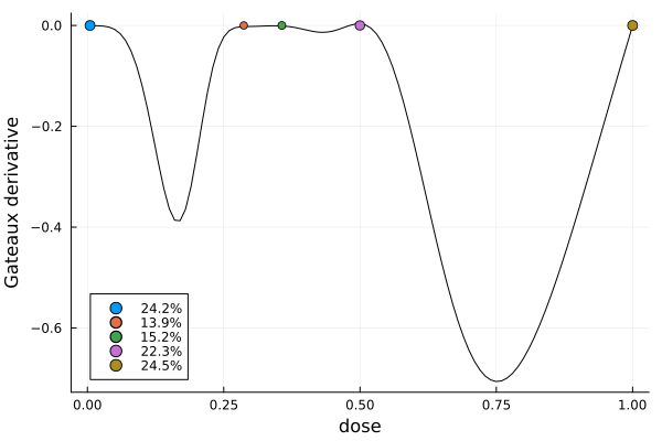
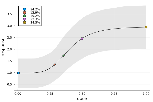
To visualize where the design points end up on the prior expected mean function, we can use plot_expected_function.
mu(dose, p) = p.e0 + p.emax * dose^p.h / (p.ed50^p.h + dose^p.h)
ef = plot_expected_function(
    (x, c, p) -> mu(x, p),     # response for fixed covariate (ignored here) and parameter
    c -> [c.dose],             # x-coordinate(s) for a point
    (c, p) -> [mu(c.dose, p)], # y-coordinate(s) for a point
    0:0.01:1,                  # x-axis grid
    s2,
    model(dp),
    covariate_parameterization(dp),
    prior_knowledge(dp);
    xguide = "dose",
    yguide = "response",
    bands = true,              # prior credible bands, by default 80%
)
Finally, we can also look at a plot of the optimization progress and see that the particle swarm has converged already after about 20 iterations.
pr1 = plot(r1)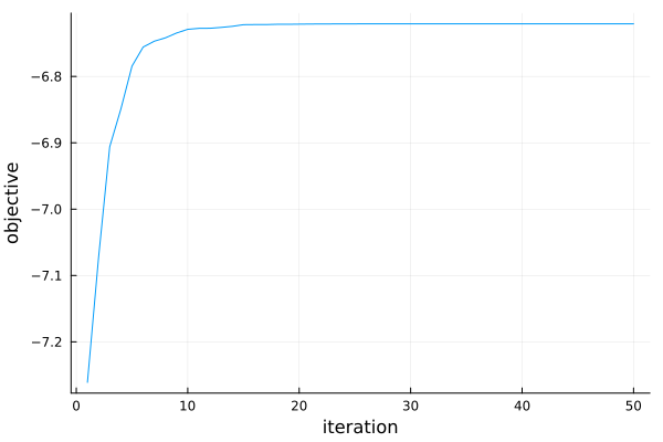
Relative Efficiency and Apportionment
In order to be able to estimate $\Parameter$ at all, we need a design with at least 4 points. Let's compare how much better the optimal solution s2 is than a 4-point equidistant_design.
efficiency(equidistant_design(dr, 4), s2, dp)0.7269868089969024Their relative D-efficiency means that s2 on average only needs 0.72 as many observations as the equidistant design with 4 points in order to achieve the same estimation accuracy.
Suppose we now actually want to run the experiment on $\SampleSize=42$ units. For this we need to convert the weights of s1 to integers that add up to $\SampleSize$. This is achieved with the apportion function:
app = apportion(s2, 42)5-element Vector{Int64}:
10
6
7
9
10This tells us to take 10 measurements at the first design point, 6 at the second, 7 at the third, and so on.