New Model Supertype
Kirstine.jl comes with support for nonlinear regression models. The theory of optimal design is of course applicable also to other regression settings. This vignette explains how to extend Kirstine.jl so that we can also find optimal designs for logistic regression.
The statistical model is
\[\begin{align*} \Unit_{\IndexUnit} \mid π_{\IndexUnit} &\simiid \BernoulliDist(π_{\IndexUnit}) \\ \Logit(π_{\IndexUnit}) &= ν(\Covariate_{\IndexUnit}, \Parameter). \end{align*}\]
Since we allow the predictor to be a nonlinear function $ν : \CovariateSet × \ParameterSet → \Reals$, our setup is more general the usual logistic GLM where the predictor is linear.
Now, we need to find the Fisher information matrix of the model. With the log-likelihood
\[\LogLikelihood(\Unit,\Covariate,\Parameter) = \Unit \log(\Expit(ν(\Covariate, \Parameter))) + (1 - \Unit) \log(1 - \Expit(ν(\Covariate, \Parameter)))\]
and some calculations we arrive at
\[- \Expectation[\Hessian\LogLikelihood\mid\Parameter] = \Expit(ν) (1 - \Expit(ν)) \TotalDiff ν' \TotalDiff ν.\]
Implementation
First we introduce a new subtype of Kirstine.Model, and a corresponding ModelWorkspace to hold the preallocated Jacobian matrix of the predictor. Then we implement a method for average_fishermatrix! that specializes on logistic regression models and returns the upper triangle of the averaged Fisher matrices.
If we had any expressions that depend on $\Covariate$, but not on $\Parameter$, we could store them in additional fields of the ModelWorkspace and compute them in update_model_workspace.
using Kirstine, Plots, Random
import LinearAlgebra: BLAS

abstract type LogisticRegression <: Kirstine.Model end

# We can define this on the supertype since it will always be the case.
Kirstine.unit_length(m::LogisticRegression) = 1

struct LRWorkspace <: Kirstine.ModelWorkspace
    jm_predictor::Matrix{Float64}
end

# We can ignore the number of design points `K` here.
function Kirstine.allocate_model_workspace(
    K::Integer,
    m::LogisticRegression,
    pk::PriorSample,
)
    return LRWorkspace(zeros(1, dimension(parameters(pk)[1])))
end

# nothing to do
function Kirstine.update_model_workspace!(
    mw::LRWorkspace,
    m::LogisticRegression,
    c::AbstractVector{<:Kirstine.Covariate},
)
    return mw
end

expit(x) = 1 / (1 + exp(-x))

function Kirstine.average_fishermatrix!(
    afm::AbstractMatrix{<:Real},
    mw::LRWorkspace,
    w::AbstractVector,
    m::LogisticRegression,
    c::AbstractVector{<:Kirstine.Covariate},
    p::Kirstine.Parameter,
)
    fill!(afm, 0.0)
    for k in 1:length(w)
        # We need to implement the next two functions for concrete subtypes.
        predictor_jacobianmatrix!(mw.jm_predictor, m, c[k], p)
        prob = expit(nonlinear_predictor(m, c[k], p))
        p1mp = prob * (1 - prob)
        BLAS.syrk!('U', 'T', p1mp * w[k], mw.jm_predictor, 1.0, afm)
    end
    return afm
end
The call to BLAS.syrk! is a more efficient way to compute
afm .+= p1mp * w[k] * mw.jm_predictor' * mw.jm_predictorin-place. Since the result is symmetric, only the upper triangle of afm is filled.
Examples
Linear Predictor
We start with a linear predictor and a $c$-dimensional covariate
\[ν(\Covariate, \Parameter) = β₀ + \sum_{j=1}^c β_j x_j\]
where $\Parameter = (β_0, β_1, …, β_c)$.
struct LinLogReg <: LogisticRegression
    dim_covariate::Int64
end

mutable struct LLRCovariate <: Kirstine.Covariate
    x::Vector{Float64}
end

Kirstine.allocate_covariate(m::LinLogReg) = LLRCovariate(zeros(m.dim_covariate))

struct LLRParameter <: Kirstine.Parameter
    beta_0::Float64
    beta_rest::Vector{Float64}
end

Kirstine.dimension(p::LLRParameter) = length(p.beta_rest) + 1

struct CopyVector <: Kirstine.CovariateParameterization end

function Kirstine.map_to_covariate!(c::LLRCovariate, dp, m::LinLogReg, cp::CopyVector)
    if length(dp) != length(c.x)
        error("dimension of covariate and design point don't match")
    end
    c.x .= dp
    return c
end

function nonlinear_predictor(m::LinLogReg, c::LLRCovariate, p::LLRParameter)
    dim_c = length(c.x)
    if length(p.beta_rest) != dim_c
        error("dimensions of covariate and parameter don't match")
    end
    np = p.beta_0
    for j in 1:dim_c
        np += p.beta_rest[j] * c.x[j]
    end
    return np
end

function predictor_jacobianmatrix!(jm, m::LinLogReg, c::LLRCovariate, p::LLRParameter)
    dim_c = length(c.x)
    if length(p.beta_rest) != dim_c
        error("dimensions of covariate and parameter don't match")
    end
    jm[1, 1] = 1
    for j in 1:dim_c
        jm[1, j + 1] = c.x[j]
    end
    return jm
end
1-Dimensional Covariate
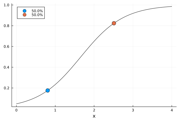
First, let's look at a locally optimal, 1-dimensional example from Section 6.2, p. 154 of [FL13], where
\[\begin{align*} \DesignRegion &= \CovariateSet = [0, 4] \\ \Parameter &= (-3, 1.81) \end{align*}\]
dp0 = DesignProblem(
    criterion = DCriterion(),
    region = DesignInterval(:x1 => (0, 4)),
    covariate_parameterization = CopyVector(),
    prior_knowledge = PriorSample([LLRParameter(-3, [1.81])]),
    model = LinLogReg(1),
)

Random.seed!(12345)
str0 = DirectMaximization(
    optimizer = Pso(swarmsize = 100, iterations = 50),
    prototype = random_design(region(dp0), 4),
)

Random.seed!(12345)
s0, r0 = solve(dp0, str0; maxdist = 1e-3)
s0
DesignMeasure(
[0.8047475621673699] => 0.49999389060536853,
[2.5101732141323296] => 0.5000061093946315,
)gd0 = plot_gateauxderivative(s0, dp0)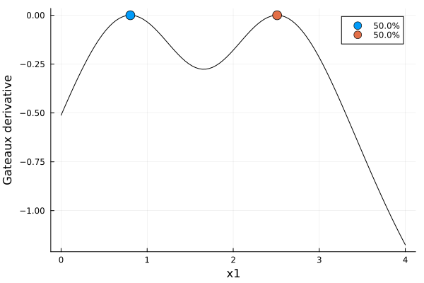
er0 = plot_expected_function(
    (x, c, p) -> expit(p.beta_0 + p.beta_rest[1] * x),
    c -> [c.x[1]],
    (c, p) -> [expit(p.beta_0 + p.beta_rest[1] * c.x[1])],
    range(lowerbound(region(dp0))[1], upperbound(region(dp0))[1]; length = 101),
    s0,
    model(dp0),
    covariate_parameterization(dp0),
    prior_knowledge(dp0);
    xguide = "x",
)
2-Dimensional Covariate
Next, we are looking at a 2-dimensional design that is locally optimal for estimating the odds ratios
\[\Transformation(\Parameter) = (\exp(β₁), \exp(β₂))'.\]
when
\[\begin{align*} \DesignRegion &= \CovariateSet = [0, 1]^2 \\ \Parameter &= (-4, 6, -3) \end{align*}\]
dp1 = DesignProblem(
    criterion = DCriterion(),
    region = DesignInterval(:x1 => (0, 1), :x2 => (0, 1)),
    covariate_parameterization = CopyVector(),
    prior_knowledge = PriorSample([LLRParameter(-4, [6, -3])]),
    model = LinLogReg(2),
    transformation = DeltaMethod(p -> [0 exp(p.beta_rest[1]) 0; 0 0 exp(p.beta_rest[2])]),
)

Random.seed!(12345)
str1 = DirectMaximization(
    optimizer = Pso(swarmsize = 100, iterations = 50),
    prototype = random_design(region(dp1), 4),
)

Random.seed!(12345)
s1, r1 = solve(dp1, str1; maxdist = 5e-2, maxweight = 1e-3)
gd1 = plot_gateauxderivative(s1, dp1)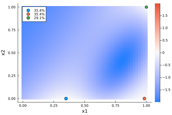
function erplot1(d, dp)
    f1(x, c, p) = expit(p.beta_0 + p.beta_rest[1] * x + p.beta_rest[2] * c.x[2])
    f2(x, c, p) = expit(p.beta_0 + p.beta_rest[1] * c.x[1] + p.beta_rest[2] * x)
    g1(c) = [c.x[1]]
    g2(c) = [c.x[2]]
    h(c, p) = [expit(p.beta_0 + p.beta_rest[1] * c.x[1] + p.beta_rest[2] * c.x[2])]
    xrange = range(lowerbound(region(dp))[1], upperbound(region(dp))[1]; length = 101)
    cp = covariate_parameterization(dp)
    pk = prior_knowledge(dp)
    m = model(dp)
    p1 = plot_expected_function(f1, g1, h, xrange, d, m, cp, pk; xguide = "x1")
    p2 = plot_expected_function(f2, g2, h, xrange, d, m, cp, pk; xguide = "x2")
    return plot(p1, p2)
end

er1 = erplot1(s1, dp1)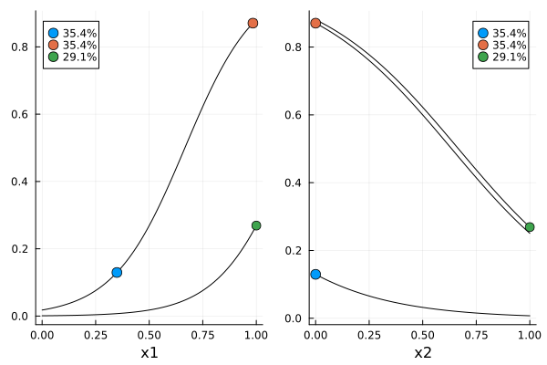
Nonlinear Predictor
A slightly silly example.
\[ν(\Covariate, \Parameter) = a \sin(2π b (t - c))\]
where $\Covariate = t$ and $\Parameter = (a, b, c)$ with $a > 0$, $b > 0$ and $0 ≤ c < 1$. We are interested in estimating all of $\Parameter$.
struct SinLogReg <: LogisticRegression end

mutable struct Time <: Kirstine.Covariate
    t::Float64
end

Kirstine.allocate_covariate(m::SinLogReg) = Time(0)

@simple_parameter SLR a b c

function nonlinear_predictor(m::SinLogReg, c::Time, p::SLRParameter)
    return p.a * sin(2 * pi * p.b * (c.t - p.c))
end

function predictor_jacobianmatrix!(jm, m::SinLogReg, c::Time, p::SLRParameter)
    sin_term = sin(2 * pi * p.b * (c.t - p.c))
    cos_term = cos(2 * pi * p.b * (c.t - p.c))
    jm[1, 1] = sin_term
    jm[1, 2] = p.a * cos_term * 2 * pi * (c.t - p.c)
    jm[1, 3] = -p.a * cos_term * 2 * pi * p.b
    return jm
end

function erplot2(d, dp)
    f(x, c, p) = expit(p.a * sin(2 * pi * p.b * (x - p.c)))
    g(c) = [c.t]
    h(c, p) = [expit(p.a * sin(2 * pi * p.b * (c.t - p.c)))]
    xrange = range(lowerbound(region(dp))[1], upperbound(region(dp))[1]; length = 101)
    cp = covariate_parameterization(dp)
    pk = prior_knowledge(dp)
    m = model(dp)
    return plot_expected_function(f, g, h, xrange, d, m, cp, pk; xguide = "time")
end

dp2 = DesignProblem(
    criterion = DCriterion(),
    region = DesignInterval(:t => (0, 1)),
    covariate_parameterization = CopyTo(:t),
    prior_knowledge = PriorSample([SLRParameter(a = 1, b = 1.5, c = 0.125)]),
    model = SinLogReg(),
)

Random.seed!(12345)
str2 = DirectMaximization(
    optimizer = Pso(swarmsize = 100, iterations = 50),
    prototype = random_design(region(dp2), 4),
)

Random.seed!(12345)
s2, r2 = solve(dp2, str2; maxdist = 5e-2, maxweight = 1e-3)
gd2 = plot_gateauxderivative(s2, dp2)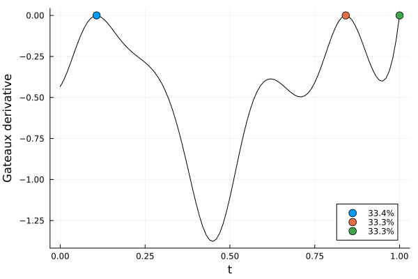
er2 = erplot2(s2, dp2)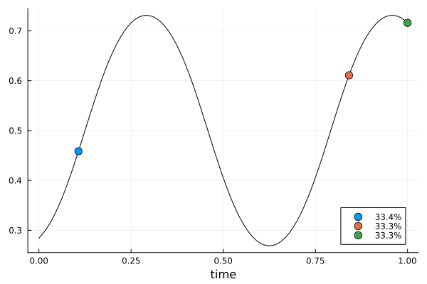
- FL13Valerii V. Fedorov and Sergei L. Leonov (2013). Optimal design for nonlinear response models. CRC Press. doi:10.1201/b15054