Discrete Priors With Nonuniform Weights
Sometimes prior knowledge is not described by a continuous distribution, which we approximately average over by Monte-Carlo integration, but by a genuinely discrete distribution. This vignette illustrates how a PriorSample can be used as an exact representation of such a discrete prior.
Model Setup
For simplicity, we reuse the dose-response model from the tutorial.
using Kirstine, Random, Plots

@simple_model SigEmax dose
@simple_parameter SigEmax e0 emax ed50 h

function Kirstine.jacobianmatrix!(
    jm,
    m::SigEmaxModel,
    c::SigEmaxCovariate,
    p::SigEmaxParameter,
)
    dose_pow_h = c.dose^p.h
    ed50_pow_h = p.ed50^p.h
    A = dose_pow_h / (dose_pow_h + ed50_pow_h)
    B = ed50_pow_h * p.emax / (dose_pow_h + ed50_pow_h)
    jm[1, 1] = 1.0
    jm[1, 2] = A
    jm[1, 3] = -A * B * p.h / p.ed50
    jm[1, 4] = c.dose == 0 ? 0.0 : A * B * log(c.dose / p.ed50)
    return jm
end
Prior Knowledge
The slope parameter $h$ of the sigmoid Emax model can in some situations be interpreted as the number of molecules that need to bind to a receptor in order to produce an effect.[W97] Suppose we suspect that only values of
\[h\in\{1,2,3,4\}\]
with prior probabilities $\{0.1, 0.3, 0.4, 0.2\}$ are possible. For simplicity suppose further that we know the values of the remaining elements of $\Parameter$ exactly. With a PriorSample, we can pass the vector of prior probabilities as the optional second argument.
prior = PriorSample(
    [SigEmaxParameter(e0 = 1, emax = 2, ed50 = 0.4, h = h) for h in 1:4],
    [0.1, 0.3, 0.4, 0.2],
)

dp = DesignProblem(
    criterion = DCriterion(),
    region = DesignInterval(:dose => (0, 1)),
    model = SigEmaxModel(sigma = 1),
    covariate_parameterization = CopyTo(:dose),
    prior_knowledge = prior,
)
Optimal Design
strategy = DirectMaximization(
    optimizer = Pso(iterations = 50, swarmsize = 100),
    prototype = equidistant_design(region(dp), 8),
)

Random.seed!(31415)
s1, r1 = solve(dp, strategy, maxweight = 1e-3, maxdist = 1e-2)
s1
DesignMeasure(
[0.0] => 0.17962034176078864,
[0.04461948295716912] => 0.0934736269518622,
[0.25627704567921966] => 0.23934177101306972,
[0.4958739526513957] => 0.23846947150228448,
[1.0] => 0.24909478877199498,
)gd = plot_gateauxderivative(s1, dp)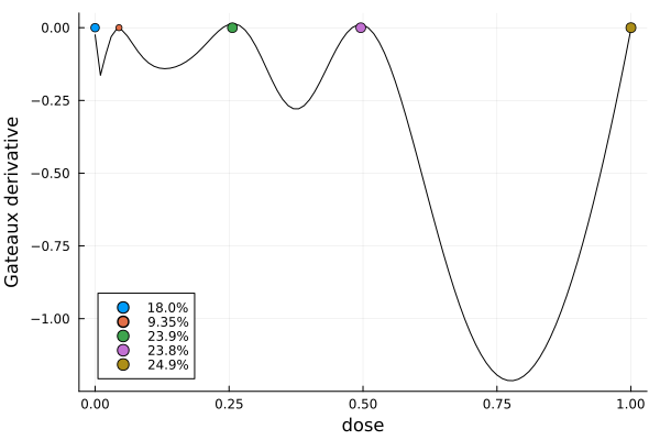
- W97James N. Weiss (1997). The hill equation revisited: uses and misuses. The FASEB Journal, 11(11), 835–841. doi:10.1096/fasebj.11.11.9285481