New Design Criterion

In this vignette, we will implement a different variant of the D-criterion. While Kirstine.jl uses

\[\DesignCriterion_D(\SomeMatrix) = \log(\det(\SomeMatrix)),\]

some authors prefer

\[\DesignCriterion_{\tilde{D}}(\SomeMatrix) = \det(\SomeMatrix)^{1/a}\]

for an $a×a$ positive definite matrix $\SomeMatrix$.

Since one criterion is a monotone bijective transformation of the other, locally optimal designs for both will be identical. But since this transformation is not linear, it can not be pulled out of the integral, and Bayesian optimal designs will be different.

For the Gateaux derivative of the objective function corresponding to $\DesignCriterion_{\tilde{D}}$ we need to compute

\[\MatDeriv{\DesignCriterion_{\tilde{D}}}{\SomeMatrix}{\SomeMatrix} = \frac{1}{a} \det(\SomeMatrix)^{1/a} \SomeMatrix^{-1}\]

which can, for example, be accomplished with the rules for matrix differential calculus from ^[MN99]. Plugging this into the general expressions we obtain

\[\begin{aligned} A &= \frac{1}{\DimTransformedParameter} \det(\TNIMatrix(\DesignMeasure, \Parameter))^{1/\DimTransformedParameter} \NIMatrix^{-1}(\DesignMeasure, \Parameter) (\TotalDiff \Transformation(\Parameter))' \TNIMatrix(\DesignMeasure, \Parameter) (\TotalDiff \Transformation(\Parameter)) \NIMatrix^{-1}(\DesignMeasure, \Parameter) \\ \Trace[B] &= \det(\TNIMatrix(\DesignMeasure, \Parameter))^{1/\DimTransformedParameter} \end{aligned}\]

for general transformations $\Transformation$, and

\[\begin{aligned} A &= \frac{1}{\DimParameter} \det(\NIMatrix(\DesignMeasure, \Parameter))^{1/\DimParameter} \NIMatrix^{-1}(\DesignMeasure, \Parameter) \\ \Trace[B] &= \det(\NIMatrix(\DesignMeasure, \Parameter))^{1/\DimParameter} \end{aligned}\]

for the special case $\Transformation(\Parameter)=\Parameter$.

Implementation

When a new T <: Kirstine.DesignCriterion is going to be used, it needs a corresponding U <: GateauxConstants which wraps precomputed values for all expressions that do not depend on the direction of the Gateaux derivative. Additionally, the following methods must be implemented.

• criterion_functional!(tnim, is_inv::Bool, dc::T): The function $\DesignCriterion$ in the mathematical notation. This function should be fast. Ideally, it should not allocate new memory.
• gateaux_constants!(<internal structures>, d::DesignMeasure, <problem parts>): Compute the value of A and tr_B of the Gateaux derivative for every parameter value in the Monte-Carlo sample. This function does a lot of in-place linear algebra with low-level pre-allocated structures. If you do not intend to use the (currently experimental) Kirstine.FrankWolfe optimizer, you can alternatively implement a slower version gateaux_constants(d::DesignMeasure, dp::DesignProblem{T,<:DesignRegion,<:Model,<:CovariateParameterization,<:Parameter,V,<:NormalApproximation}) that dispatches on your new criterion type T and either V=Identity or V=DeltaMethod. It should allocate and return a Kirstine.GCPriorSample.

Next, we will implement the alternative D-criterion for Identity and DeltaMethod transformations. Since it is in some way the exponential of the predefined version, we will call it DexpCriterion.

using Kirstine
using LinearAlgebra: Symmetric, det
using LinearAlgebra.LAPACK: potri!, posv!
using LinearAlgebra.BLAS: gemm!

struct DexpCriterion <: Kirstine.DesignCriterion end

# `tnim` is the transformed normalized information matrix.
# It is implicitly symmetric, i.e. only the upper triangle contains sensible values.
# Depending on the transformation used, `tnim` can stand for M_(ζ,θ) or M_(ζ,θ)^{-1}.
# The information about this is passed in the `is_inv` flag.
# `log_det!` computes `log(det())` of its argument, treating it as implicitly symmetric
# and overwriting it in the process.
function Kirstine.criterion_functional!(
    tnim::AbstractMatrix,
    is_inv::Bool,
    dc::DexpCriterion,
)
    sgn = is_inv ? -1 : 1
    ld = Kirstine.log_det!(tnim)
    # `tnim` could be singular. In such a case the corresponding design measure can't be a solution.
    # Hence we do not want to accidentally flip the sign then.
    cv = ld != -Inf ? sgn * ld : ld
    t = size(tnim, 1)
    return exp(cv / t)
end

function Kirstine.gateaux_constants!(
    gc::Kirstine.GCPriorSample,
    mw::Kirstine.ModelWorkspace,
    nw::Kirstine.NIMWorkspace,
    c::AbstractVector{<:Kirstine.Covariate},
    dc::DexpCriterion,
    d::DesignMeasure,
    m::Kirstine.Model,
    cp::Kirstine.CovariateParameterization,
    pk::PriorSample,
    tc::Kirstine.TCIdentity,
    na::Kirstine.NormalApproximation,
)
    ps = parameters(pk)
    r = dimension(ps[1])
    Kirstine.update_covariates!(c, d, m, cp)
    Kirstine.update_model_workspace!(mw, m, c)
    for i in 1:length(ps)
        Kirstine.average_fishermatrix!(nw.r_x_r, mw, weights(d), m, c, ps[i])
        Kirstine.informationmatrix!(nw.r_x_r, na)
        # tr_B := det(M)^(1/r)
        gc.tr_B[i] = exp(Kirstine.log_det!(nw.r_x_r) / r) # performs potrf!() internally
        # nw.r_x_r := inv(M)
        potri!('U', nw.r_x_r)
        # nw.r_x_r := (1/r) * det(M)^(1/r) * inv(M)
        nw.r_x_r .*= gc.tr_B[i] / r
        gc.A[i] .= nw.r_x_r # only upper triangle
    end
    return gc
end

function Kirstine.gateaux_constants!(
    gc::Kirstine.GCPriorSample,
    mw::Kirstine.ModelWorkspace,
    nw::Kirstine.NIMWorkspace,
    c::AbstractVector{<:Kirstine.Covariate},
    dc::DexpCriterion,
    d::DesignMeasure,
    m::Kirstine.Model,
    cp::Kirstine.CovariateParameterization,
    pk::PriorSample,
    tc::Kirstine.TCDeltaMethod,
    na::Kirstine.NormalApproximation,
)
    r = size(nw.r_x_r, 1)
    t = size(nw.t_x_t, 1)
    ps = parameters(pk)
    Kirstine.update_covariates!(c, d, m, cp)
    Kirstine.update_model_workspace!(mw, m, c)
    for i in 1:length(ps)
        Kirstine.average_fishermatrix!(nw.r_x_r, mw, weights(d), m, c, ps[i])
        Kirstine.informationmatrix!(nw.r_x_r, na)
        gc.A[i] .= nw.r_x_r # store it temporarily here, apply_transformation!() will overwrite it
        # nw.t_x_t := inv(Q)
        nw.r_is_inv = false
        Kirstine._apply_transformation_delta!(nw, tc.jm[i])
        # nw.r_x_t := inv(M) * DT'
        nw.r_x_t .= tc.jm[i]'
        posv!('U', gc.A[i], nw.r_x_t)
        # nw.t_x_r := DT * inv(M)
        nw.t_x_r .= nw.r_x_t'
        # nw.t_x_r := Q * DT * inv(M) and implicitly nw.t_x_t := upper cholesky factor of inv(Q)
        posv!('U', nw.t_x_t, nw.t_x_r)
        # tr_B = det(Q)^(1/t)
        gc.tr_B[i] =
            exp(-2 * sum(nw.t_x_t[j, j] > 0 ? log(nw.t_x_t[j, j]) : -Inf for j in 1:t) / t)
        # nw.r_x_r := inv(M) * DT' * Q * DT * inv(M)
        gemm!('N', 'N', 1.0, nw.r_x_t, nw.t_x_r, 0.0, nw.r_x_r)
        # A := (1/t) * det(Q)^(1/t) * inv(M) * DT' * Q * DT * inv(M)
        gc.A[i] .= nw.r_x_r .* gc.tr_B[i] / t # dense
    end
    return gc
end

Example

For illustration, we re-use the discrete prior example.

using Random, Plots

@simple_model SigEmax dose
@simple_parameter SigEmax e0 emax ed50 h

function Kirstine.jacobianmatrix!(
    jm,
    m::SigEmaxModel,
    c::SigEmaxCovariate,
    p::SigEmaxParameter,
)
    dose_pow_h = c.dose^p.h
    ed50_pow_h = p.ed50^p.h
    A = dose_pow_h / (dose_pow_h + ed50_pow_h)
    B = ed50_pow_h * p.emax / (dose_pow_h + ed50_pow_h)
    jm[1, 1] = 1.0
    jm[1, 2] = A
    jm[1, 3] = -A * B * p.h / p.ed50
    jm[1, 4] = c.dose == 0 ? 0.0 : A * B * log(c.dose / p.ed50)
    return jm
end

prior = PriorSample(
    [SigEmaxParameter(e0 = 1, emax = 2, ed50 = 0.4, h = h) for h in 1:4],
    [0.1, 0.3, 0.4, 0.2],
)

We compute D-optimal designs under both variants of the criterion, once for estimating the full parameter, and once for only estimating ed50 and h.

dp1a = DesignProblem(
    criterion = DexpCriterion(),
    region = DesignInterval(:dose => (0, 1)),
    model = SigEmaxModel(sigma = 1),
    covariate_parameterization = JustCopy(:dose),
    prior_knowledge = prior,
)

dp1b = DesignProblem(dp1a; criterion = DCriterion())

dp2a = DesignProblem(dp1a; transformation = DeltaMethod(p -> [0 0 1 0; 0 0 0 1]))

dp2b = DesignProblem(
    dp1a;
    criterion = DCriterion(),
    transformation = DeltaMethod(p -> [0 0 1 0; 0 0 0 1]),
)

strategy = DirectMaximization(
    optimizer = Pso(iterations = 50, swarmsize = 100),
    prototype = equidistant_design(region(dp1a), 8),
)

Random.seed!(31415)
s1a, r1a = solve(dp1a, strategy, maxweight = 1e-3, maxdist = 1e-2)
Random.seed!(31415)
s1b, r1b = solve(dp1b, strategy, maxweight = 1e-3, maxdist = 1e-2)
Random.seed!(31415)
s2a, r2a = solve(dp2a, strategy, maxweight = 1e-3, maxdist = 1e-2)
Random.seed!(31415)
s2b, r2b = solve(dp2b, strategy, maxweight = 1e-3, maxdist = 1e-2)

gd1 = plot(
    plot_gateauxderivative(s1a, dp1a; title = "1a"),
    plot_gateauxderivative(s2a, dp2a; title = "2a"),
    plot_gateauxderivative(s1b, dp1b; title = "1b"),
    plot_gateauxderivative(s2b, dp2b; title = "2b"),
)

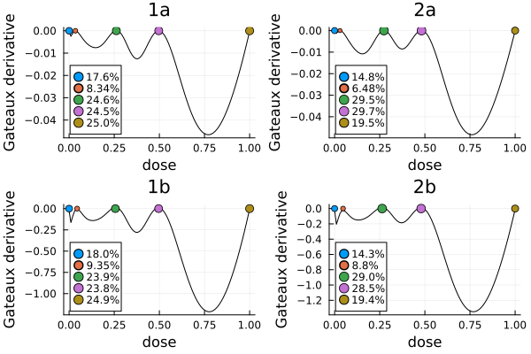
The solutions under both D-criterion variants are rather similar

[reduce(vcat, points(s2a)) reduce(vcat, points(s2b))]

5×2 Matrix{Float64}:
 0.0        0.0
 0.0297763  0.0467735
 0.2733     0.263581
 0.481463   0.479369
 1.0        1.0

[reduce(vcat, points(s2a)) reduce(vcat, points(s2b))]

5×2 Matrix{Float64}:
 0.0        0.0
 0.0297763  0.0467735
 0.2733     0.263581
 0.481463   0.479369
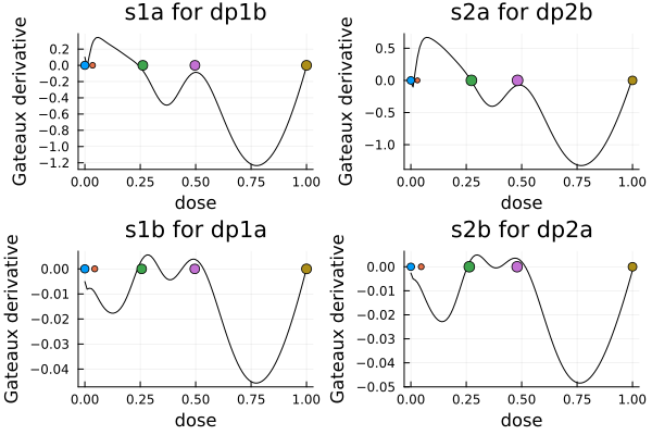
 1.0        1.0

but not the same

gd2 = plot(
    plot_gateauxderivative(s1a, dp1b; title = "s1a for dp1b", legend = nothing),
    plot_gateauxderivative(s2a, dp2b; title = "s2a for dp2b", legend = nothing),
    plot_gateauxderivative(s1b, dp1a; title = "s1b for dp1a", legend = nothing),
    plot_gateauxderivative(s2b, dp2a; title = "s2b for dp2a", legend = nothing),
)