New Problem Solving Strategy
On a high level, Kirstine.jl can use different Kirstine.ProblemSolvingStrategys to find the solution to a design problem. The package implements DirectMaximization and a version of Fedorov's Exchange algorithm. This vignette shows how to implement a custom strategy.
Our example will be a variant of direct maximization that runs the given Kirstine.Optimizer multiple times, using the best candidate from the current iteration as the prototype for initializing the next one. A further extension of this example could also include a check of the Gateaux derivative for early stopping.
Implementation
For a Ts <: Kirstine.ProblemSolvingStrategy we need a corresponding Tr <: Kirstine.ProblemSolvingResult, plus methods for the following functions:
solve_with(adp::AbstractDesignProblem, strategy::Ts, trace_state::Bool)which does the actual work and returns aTr. The flagtrace_stateshould passed to the low-levelKirstine.Optimizer.solution(res::Tr)to extract the best solution that was found.total_runtime(res::Tr)to extract the total runtime in seconds.
Optionally, for producing a plot of the optimization progress, we can also implement a type recipe for Tr. When it comes to plotting a Vector of Kirstine.OptimizationResults, Kirstine.jl already provides a basic recipe that we can reuse.
For simplicity we require the low-level optimizer to be of order zero.
using Kirstine, RecipesBase, Plots

struct MultipleRuns{T<:Kirstine.ZerothOrderOptimizer} <: Kirstine.ProblemSolvingStrategy
    optimizer::T
    prototype::DesignMeasure
    steps::Int64
    fixedweights::Vector{Int64}
    fixedpoints::Vector{Int64}
    function MultipleRuns(;
        optimizer::T,
        prototype::DesignMeasure,
        steps::Integer,
        fixedweights::AbstractVector{<:Integer} = Int64[],
        fixedpoints::AbstractVector{<:Integer} = Int64[],
    ) where T<:Kirstine.ZerothOrderOptimizer
        new{T}(optimizer, prototype, steps, fixedweights, fixedpoints)
    end
end

struct MultipleRunsResult{
    S<:Kirstine.OptimizerState{DesignMeasure,Kirstine.SignedMeasure},
} <: Kirstine.ProblemSolvingResult
    ors::Vector{Kirstine.OptimizationResult{DesignMeasure,Kirstine.SignedMeasure,S}}
end

function Kirstine.solution(mrr::MultipleRunsResult)
    return mrr.ors[end].maximizer
end

function Kirstine.total_runtime(mrr::MultipleRunsResult)
    return mapreduce(or -> or.seconds_elapsed, +, mrr.ors)
end

function Kirstine.solve_with(
    adp::Kirstine.AbstractDesignProblem,
    strategy::MultipleRuns,
    trace_state::Bool,
)
    # `Kirstine.optimize()` needs to know the constraints for the optimization problem.
    constraints = Kirstine.DesignConstraints(
        strategy.prototype,
        region(adp),
        strategy.fixedweights,
        strategy.fixedpoints,
    )
    # set up preallocated objects for the objective function to work on
    oc = Kirstine.objective_constants(adp)
    w = Kirstine.allocate_workspace(strategy.prototype, adp)
    optimization_helper(prototype) = Kirstine.optimize(
        d -> Kirstine.objective!(w, d, adp, oc),
        strategy.optimizer,
        [prototype],
        constraints;
        trace_state = trace_state,
    )

    # initial run
    ors = [optimization_helper(strategy.prototype)]

    # subsequent runs
    for i in 2:(strategy.steps)
        new_prototype = ors[i - 1].maximizer
        or = optimization_helper(new_prototype)
        push!(ors, or)
    end
    return MultipleRunsResult(ors)
end

@recipe function f(r::MultipleRunsResult)
    return r.ors # just need to unwrap
end
Example
Again, we use the discrete prior example.
using Kirstine, Random, Plots

@simple_model SigEmax dose
@simple_parameter SigEmax e0 emax ed50 h

function Kirstine.jacobianmatrix!(
    jm,
    m::SigEmaxModel,
    c::SigEmaxCovariate,
    p::SigEmaxParameter,
)
    dose_pow_h = c.dose^p.h
    ed50_pow_h = p.ed50^p.h
    A = dose_pow_h / (dose_pow_h + ed50_pow_h)
    B = ed50_pow_h * p.emax / (dose_pow_h + ed50_pow_h)
    jm[1, 1] = 1.0
    jm[1, 2] = A
    jm[1, 3] = -A * B * p.h / p.ed50
    jm[1, 4] = c.dose == 0 ? 0.0 : A * B * log(c.dose / p.ed50)
    return jm
end

prior = PriorSample(
    [SigEmaxParameter(e0 = 1, emax = 2, ed50 = 0.4, h = h) for h in 1:4],
    [0.1, 0.3, 0.4, 0.2],
)

dp = DesignProblem(
    criterion = DCriterion(),
    region = DesignInterval(:dose => (0, 1)),
    model = SigEmaxModel(sigma = 1),
    covariate_parameterization = CopyTo(:dose),
    prior_knowledge = prior,
)

strategy = MultipleRuns(
    optimizer = Pso(iterations = 20, swarmsize = 25),
    prototype = equidistant_design(region(dp), 8),
    steps = 10,
)

Random.seed!(31415)
s, r = solve(dp, strategy, maxweight = 1e-3, maxdist = 1e-2)
gd = plot_gateauxderivative(s, dp)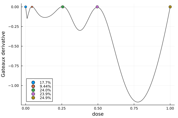
total_runtime(r)0.07813906669616699pr = plot(r)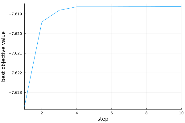
We see that the solution was found after four steps.