Optimal Design for Functions of the Parameter

This vignette shows how to find a D-optimal design for estimating some transformation $\Transformation(\Parameter)$ of the model parameter. The function $\Transformation : \ParameterSet → \Reals^{\DimTransformedParameter}$ must be differentiable with a full-rank Jacobian matrix.

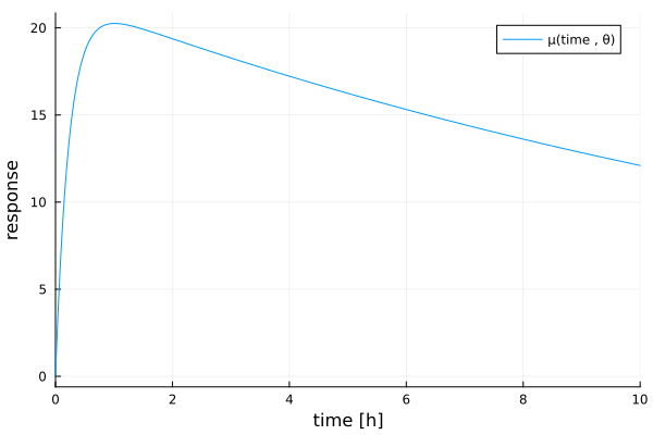
Our example in this vignette is the three-parameter compartment model from Atkinson et al^[ACHJ93]. In pharmacokinetics, it describes how the concentration of a drug in an experimental subject changes over time. The mean function for the regression is given by

\[\MeanFunction(\Covariate, \Parameter) = s (\exp(-e\Covariate) - \exp(-a\Covariate))\]

where the elements of $\Parameter$ are the absorption rate $a$, the elimination rate $e$, and a scaling factor $s$. The covariate $\Covariate$ denotes the time in hours.

θ = (a = 4.298, e = 0.05884, s = 21.80)
tpc = plot(
    x -> θ.s * (exp(-θ.e * x) - exp(-θ.a * x));
    xlims = (0, 10),
    xguide = "time [h]",
    yguide = "response",
    label = "μ(time , θ)",
)

Setup

As in the introductory example, we start by defining the (single-row) Jacobian matrix of the mean function, and the mapping from design variables to model covariates.

using Kirstine, Plots, Random, Statistics

@simple_model TPC time
@simple_parameter TPC a e s

function Kirstine.jacobianmatrix!(jm, m::TPCModel, c::TPCCovariate, p::TPCParameter)
    A = exp(-p.a * c.time)
    E = exp(-p.e * c.time)
    jm[1, 1] = A * p.s * c.time
    jm[1, 2] = -E * p.s * c.time
    jm[1, 3] = E - A
    return m
end

In this vignette we will only look at Bayesian optimal designs because locally optimal designs for scalar $\Transformation(\Parameter)$ usually don't exist due to their information matrices becoming singular.

For the prior we will use “distribution I” from^[ACHJ93], which is constructed from two independent uniform distributions around estimates for $a$ and $e$, and a point mass for $s$. The strength of the prior is controlled by the width of the uniform distributions. We generate a PriorSample from 1000 draws.

function draw_from_prior(n, se_factor)
    mn = [4.298, 0.05884, 21.8]
    se = [0.5, 0.005, 0]
    as = mn[1] .+ se_factor .* se[1] .* (2 .* rand(n) .- 1)
    es = mn[2] .+ se_factor .* se[2] .* (2 .* rand(n) .- 1)
    ss = mn[3] .+ se_factor .* se[3] .* (2 .* rand(n) .- 1)
    return PriorSample(map((a, e, s) -> TPCParameter(a = a, e = e, s = s), as, es, ss))
end

In this vignette we will focus on the effect of different transformations. We start with the following design problem and replace its transformation as needed. Our design interval extends from 0 to 48 hours after administration of the drug. We set the seed to get a reproducible draw from the prior.

Random.seed!(4711)
dp_id = DesignProblem(
    region = DesignInterval(:time => [0, 48]),
    criterion = DCriterion(),
    covariate_parameterization = CopyTo(:time),
    model = TPCModel(sigma = 1),
    prior_knowledge = draw_from_prior(1000, 2),
    transformation = Identity(),
)

In all subsequent examples we will use identical settings for the particle swarm optimizer, and start with an equidistant design.

pso = Pso(swarmsize = 50, iterations = 100)
dms = DirectMaximization(optimizer = pso, prototype = uniform_design([[0], [24], [48]]))

The following is a small wrapper around plot_expected_function that plots a time-response curve and overlays the measurement points implied by the design.

function plot_expected_response(d::DesignMeasure, dp::DesignProblem)
    response(t, p) = p.s * (exp(-p.e * t) - exp(-p.a * t))
    f(x, c, p) = response(x, p)
    g(c) = [c.time]
    h(c, p) = [response(c.time, p)]
    xrange = range(0, 48; length = 101)
    cp = covariate_parameterization(dp)
    plt = plot_expected_function(f, g, h, xrange, d, model(dp), cp, prior_knowledge(dp))
    plot!(plt; xguide = "time", yguide = "response", xticks = 0:6:48)
    return plt
end

Identity Transformation

In order to have a design to compare other solutions against, we first determine the Bayesian D-optimal design for the whole parameter $\Parameter$.

Random.seed!(1357)
s_id, r_id = solve(dp_id, dms)

s_id

DesignMeasure(
 [0.228863250498729] => 0.3333144478760726,
 [1.4181500168247514] => 0.33329978174892977,
 [18.520007438612772] => 0.33338577037499756,
)

gd_id = plot_gateauxderivative(s_id, dp_id)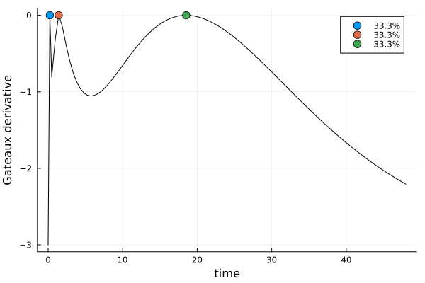

ef_id = plot_expected_response(s_id, dp_id)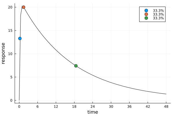

Univariate Functions

Area Under the Curve

In pharmacokinetics, one quantity of particular interest is the area under the response curve. It can be calculated as

\[\mathrm{AUC}(\Parameter) = s \bigg( \frac{1}{e} - \frac{1}{a} \bigg).\]

Suppose we want to find a design that maximizes the information about $\mathrm{AUC}(\Parameter)$. This needs an additional approximation step via the delta method, for which we need to know the Jacobian matrix of $\mathrm{AUC}$:

function Dauc(p)
    del_a = p.s / p.a^2
    del_e = -p.s / p.e^2
    del_s = 1 / p.e - 1 / p.a
    return [del_a del_e del_s]
end

Note that we return a row vector, and that the order of the partial derivatives is the same as in the Jacobian matrix of the mean function.

Now make a copy of dp_id in which we replace the Identity transformation by a DeltaMethod object that wraps the Jacobian matrix function. (This is more convenient than explicitly specifying again all the parts that should stay the same.)

dp_auc = DesignProblem(dp_id; transformation = DeltaMethod(Dauc))
Random.seed!(1357)
s_auc, r_auc = solve(dp_auc, dms)
s_auc

DesignMeasure(
 [0.24531677720907377] => 0.013165898968091254,
 [1.499218615533174] => 0.038534397924271095,
 [18.227704273038025] => 0.9482997031076377,
)

gd_auc = plot_gateauxderivative(s_auc, dp_auc)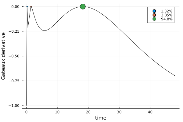

ef_auc = plot_expected_response(s_auc, dp_auc)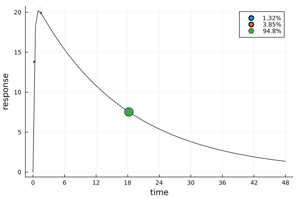

The design points are similar to those of s_id, but while its weights were practically uniform, the weight of s_auc is almost completely placed at its third design point. We can also see that s_auc is nearly three times as efficient as s_id for estimating the AUC:

efficiency(s_id, s_auc, dp_auc)

0.3702594267798839

Note that this relation is not necessarily symmetric: s_id is five times as efficient as s_auc for estimating $\Parameter$.

efficiency(s_auc, s_id, dp_id)

0.23450915325603677

Time to Maximum Concentration

Now let's find a design that is optimal for estimating the point in time where the concentration is highest. Differentiating $\MeanFunction$ with respect to $\Covariate$, equating with $0$ and solving for $\Covariate$ gives

\[t_{\max{}}(\Parameter) = \frac{\log(a / e)}{a - e}.\]

Its Jacobian matrix is

function Dttm(p)
    A = p.a - p.e
    A2 = A^2
    B = log(p.a / p.e)
    da = (A / p.a - B) / A2
    de = (B - A / p.e) / A2
    ds = 0
    return [da de ds]
end

dp_ttm = DesignProblem(dp_id; transformation = DeltaMethod(Dttm))
Random.seed!(1357)
s_ttm, r_ttm = solve(dp_ttm, dms)
s_ttm

DesignMeasure(
 [0.1785277717204147] => 0.6022152518991615,
 [2.4347788334799083] => 0.2985274392389716,
 [8.778030603264321] => 0.09925730886186684,
)

gd_ttm = plot_gateauxderivative(s_ttm, dp_ttm)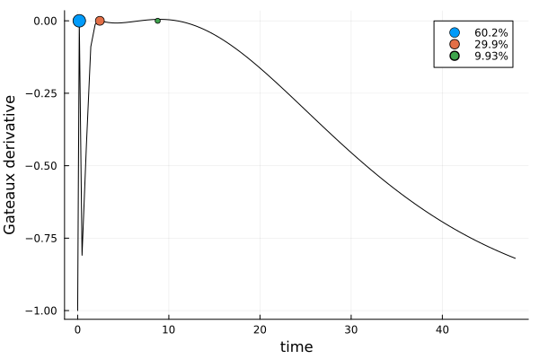

ef_ttm = plot_expected_response(s_ttm, dp_ttm)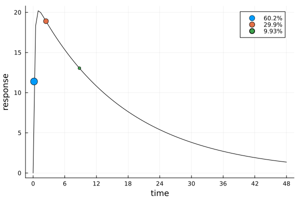

This solution differs markedly from the previous ones.

Maximum Concentration

What if we're not interested in the time of maximum concentration, but in the value of the maximum concentration $\MeanFunction(t_{\max{}}(\Parameter), \Parameter)$ itself?

ttm(p) = log(p.a / p.e) / (p.a - p.e)

function Dcmax(p)
    tmax = ttm(p)
    A = exp(-p.a * tmax)
    E = exp(-p.e * tmax)
    F = p.a * A - p.e * E
    da_ttm, de_ttm, ds_ttm = Dttm(p)
    da = p.s * (tmax * A - F * da_ttm)
    de = p.s * (-tmax * E + F * de_ttm)
    ds = E - A
    return [da de ds]
end

dp_cmax = DesignProblem(dp_id; transformation = DeltaMethod(Dcmax))
Random.seed!(13579)
s_cmax, r_cmax = solve(dp_cmax, dms)
s_cmax

DesignMeasure(
 [0.3634701770982941] => 0.07255932607971026,
 [1.14355863427162] => 0.9102152568783713,
 [20.797213533057352] => 0.01722541704191838,
)

gd_cmax = plot_gateauxderivative(s_cmax, dp_cmax)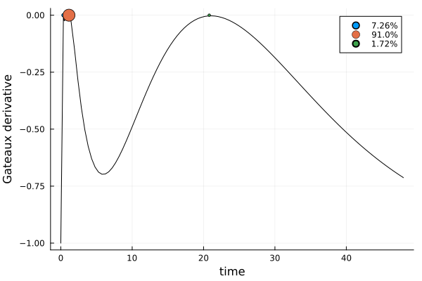

ef_cmax = plot_expected_response(s_cmax, dp_cmax)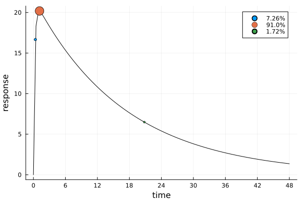

The solution is again mostly concentrated on one design point. The location of this point makes intuitive sense, considering the prior expected time to maximum concentration:

prior_expected_ttm = mean(ttm, parameters(prior_knowledge(dp_cmax)))

1.0272684144529458

Multivariate Functions

Finding D-optimal designs for vector functions of the parameter is just as easy. Suppose we are interested in both the time and the value of the maximum concentration. Because we have already defined their single Jacobian matrices, we now only need to concatenate them vertically.

Dboth(p) = [Dttm(p); Dcmax(p)]
dp_both = DesignProblem(dp_id; transformation = DeltaMethod(Dboth))
Random.seed!(1357)
s_both, r_both = solve(dp_both, dms)
s_both

DesignMeasure(
 [0.23663824657919236] => 0.4173416078008837,
 [1.3894258771295565] => 0.4978247422912806,
 [18.91391407149987] => 0.0848336499078357,
)

gd_both = plot_gateauxderivative(s_both, dp_both)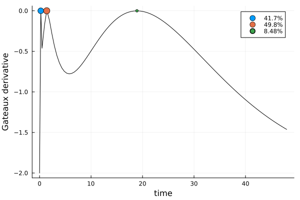

ef_both = plot_expected_response(s_both, dp_both)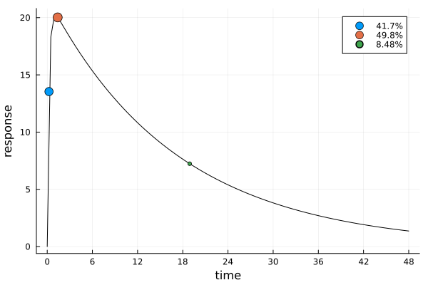

This solution is again similar to s_id, but with a different weight distribution.

Finally we compare all pairwise efficiencies (solutions in rows, transformations in columns):

solutions = [s_id, s_auc, s_ttm, s_cmax, s_both]
problems = [dp_id, dp_auc, dp_ttm, dp_cmax, dp_both]
map(Iterators.product(solutions, zip(solutions, problems))) do (s1, (s2, dp))
    efficiency(s1, s2, dp)
end

5×5 Matrix{Float64}:
 1.0       0.370259   0.669859   0.398903   0.786635
 0.234509  1.0        0.0326718  0.0449486  0.0540548
 0.569863  0.0513228  1.0        0.199012   0.658729
 0.278374  0.0187619  0.121608   1.0        0.496585
 0.780164  0.094294   0.781641   0.590004   1.0